Modeling - Clustering
Clustering
Clustering is a method which groups the "closest" values together. This page will analyze results and applications from different clustering methods. Namely, the following will be explored:
- KMeans Clustering
- Hierarchical Clustering
- DBSCAN (Density) Clustering
What Data Can Be Used?
The data for cluster modeling will be initialized with PCA. Therefore, the data preparation will be identical to the PCA section.
This analysis focuses on the quantitative data of the main datasets used throughout this project:
Ski Resorts Data - Snippet
| Resort | state_province_territory | Country | City | Overall Rating | Elevation Difference | Elevation Low | Elevation High | Trails Total | Trails Easy | Trails Intermediate | Trails Difficult | Lifts | Price | Resort Size | Run Variety | Lifts Quality | Latitude | Longitude | Pass | Region |
|---|---|---|---|---|---|---|---|---|---|---|---|---|---|---|---|---|---|---|---|---|
| 49 Degrees North Mountain Resort | Washington | United States | Chewelah | 3.4 | 564 | 1196 | 1760 | 68.0 | 20.0 | 27.0 | 21.0 | 7 | 82.0 | 3.5 | 4.0 | 3.3 | 48.277375 | -117.701815 | Other | West |
| Crystal Mountain (WA) | Washington | United States | Sunrise | 3.3 | 796 | 1341 | 2137 | 50.0 | 8.0 | 27.0 | 15.0 | 11 | 199.0 | 3.2 | 3.6 | 3.7 | 46.928167 | -121.504535 | Ikon | West |
| Mt. Baker | Washington | United States | White Salmon | 3.4 | 455 | 1070 | 1525 | 100.0 | 24.0 | 45.0 | 31.0 | 10 | 91.0 | 3.9 | 4.3 | 3.0 | 45.727775 | -121.486699 | Other | West |
| Mt. Spokane | Washington | United States | Mead | 3.0 | 610 | 1185 | 1795 | 26.0 | 6.5 | 16.0 | 3.5 | 7 | 75.0 | 2.7 | 3.1 | 3.0 | 47.919072 | -117.092505 | Other | West |
| Sitzmark | Washington | United States | Tonasket | 2.6 | 155 | 1330 | 1485 | 7.5 | 2.0 | 3.0 | 2.5 | 2 | 50.0 | 1.9 | 2.4 | 2.9 | 48.863907 | -119.165077 | Other | West |
| Stevens Pass | Washington | United States | Baring | 3.3 | 580 | 1170 | 1750 | 39.0 | 6.0 | 18.0 | 15.0 | 10 | 119.0 | 3.1 | 3.5 | 3.6 | 47.764031 | -121.474822 | Epic | West |
| The Summit at Snoqualmie | Washington | United States | Snoqualmie Pass | 3.0 | 380 | 800 | 1180 | 27.9 | 5.2 | 13.7 | 9.0 | 22 | 135.0 | 2.6 | 3.0 | 3.2 | 47.405235 | -121.412783 | Ikon | West |
| Wenatchee Mission Ridge | Washington | United States | Wenatchee | 3.2 | 686 | 1392 | 2078 | 36.0 | 4.0 | 21.0 | 11.0 | 4 | 119.0 | 2.9 | 3.3 | 3.6 | 47.292466 | -120.399871 | Other | West |
| Abenaki | New Hampshire | United States | Wolfeboro | 2.1 | 70 | 180 | 250 | 2.0 | 1.2 | 0.5 | 0.3 | 1 | 24.0 | 1.4 | 1.8 | 1.4 | 43.609528 | -71.229692 | Other | Northeast |
| Attitash Mountain Resort | New Hampshire | United States | Bartlett | 3.2 | 533 | 183 | 716 | 37.0 | 7.4 | 17.4 | 12.2 | 8 | 129.0 | 2.9 | 3.3 | 3.7 | 44.084603 | -71.221525 | Epic | Northeast |
Weather Data - Snippet
| datetime | tempmax | tempmin | temp | feelslikemax | feelslikemin | feelslike | dew | humidity | precip | precipprob | precipcover | snow | snowdepth | windgust | windspeed | winddir | pressure | cloudcover | visibility | solarradiation | solarenergy | uvindex | sunrise | sunset | moonphase | icon | stations | resort | tzoffset | severerisk | type_freezingrain | type_ice | type_none | type_rain | type_snow |
|---|---|---|---|---|---|---|---|---|---|---|---|---|---|---|---|---|---|---|---|---|---|---|---|---|---|---|---|---|---|---|---|---|---|---|---|
| 2019-01-01 | 16.4 | 2.0 | 7.0 | 10.2 | -13.3 | -0.6 | -1.2 | 69.1 | 0.008 | 100.0 | 20.83 | 0.0 | 20.7 | 18.30000 | 10.6 | 4.9 | 1014.5 | 59.0 | 8.6 | 116.8 | 9.9 | 5.0 | 07:26:20 | 16:51:51 | 0.85 | snow | ['72467523063', '72206103038', 'CACMC', 'KCCU', 'KEGE', 'KLXV', 'DJTC2', 'K20V', '72467393009'] | Vail | 0.0 | 0.0 | 0 | 0 | 0 | 0 | 1 |
| 2019-01-02 | 24.3 | -0.9 | 11.4 | 21.9 | -11.9 | 5.4 | -10.5 | 39.9 | 0.004 | 100.0 | 4.17 | 0.0 | 20.8 | 29.77377 | 8.7 | 353.1 | 1021.4 | 0.0 | 9.9 | 121.6 | 10.7 | 5.0 | 07:26:27 | 16:52:41 | 0.89 | snow | ['72467523063', '72206103038', 'CACMC', 'KCCU', 'KEGE', 'KLXV', 'DJTC2', 'K20V', '72467393009'] | Vail | 0.0 | 0.0 | 0 | 0 | 0 | 0 | 1 |
| 2019-01-03 | 29.0 | 5.3 | 17.6 | 21.9 | -4.0 | 8.6 | 4.1 | 56.1 | 0.004 | 100.0 | 4.17 | 0.2 | 20.8 | 32.20000 | 9.8 | 328.9 | 1024.7 | 0.0 | 9.8 | 123.3 | 10.6 | 5.0 | 07:26:31 | 16:53:33 | 0.92 | snow | ['72467523063', '72206103038', 'CACMC', 'KCCU', 'KEGE', 'KLXV', 'DJTC2', 'K20V', '72467393009'] | Vail | 0.0 | 0.0 | 0 | 0 | 0 | 1 | 1 |
| 2019-01-04 | 34.0 | 11.9 | 23.4 | 28.7 | 3.4 | 17.1 | 7.0 | 50.4 | 0.001 | 100.0 | 4.17 | 0.1 | 20.8 | 20.80000 | 9.0 | 311.0 | 1025.5 | 0.0 | 9.9 | 123.7 | 10.7 | 5.0 | 07:26:34 | 16:54:26 | 0.96 | snow | ['72467523063', '72206103038', 'CACMC', 'KCCU', 'KEGE', 'KLXV', 'DJTC2', 'K20V', '72467393009'] | Vail | 0.0 | 0.0 | 0 | 0 | 0 | 1 | 1 |
| 2019-01-05 | 34.1 | 14.3 | 27.1 | 29.4 | 4.3 | 20.1 | 1.9 | 33.9 | 0.001 | 100.0 | 4.17 | 0.0 | 20.4 | 20.80000 | 10.1 | 243.5 | 1022.2 | 19.4 | 9.7 | 110.3 | 9.6 | 5.0 | 07:26:34 | 16:55:20 | 0.00 | rain | ['72467523063', '72206103038', 'CACMC', 'DYGC2', 'KCCU', 'KEGE', 'KLXV', 'DJTC2', 'K20V', '72467393009'] | Vail | 0.0 | 0.0 | 0 | 0 | 0 | 1 | 1 |
| 2019-01-06 | 29.9 | 18.5 | 25.9 | 22.4 | 5.1 | 16.1 | 18.1 | 72.5 | 0.035 | 100.0 | 58.33 | 0.6 | 20.6 | 33.30000 | 16.9 | 266.7 | 1009.3 | 78.7 | 6.3 | 47.3 | 4.1 | 2.0 | 07:26:32 | 16:56:16 | 0.02 | snow | ['72467523063', '72206103038', 'CACMC', '72038500419', 'DYGC2', 'KCCU', 'KEGE', 'A0000594076', 'KLXV', 'DJTC2', 'K20V', '72467393009'] | Vail | 0.0 | 0.0 | 0 | 0 | 0 | 1 | 1 |
| 2019-01-07 | 24.8 | 14.7 | 20.3 | 12.8 | 2.5 | 6.5 | 13.7 | 75.2 | 0.004 | 100.0 | 8.33 | 0.4 | 21.3 | 45.70000 | 27.9 | 271.2 | 1015.6 | 83.7 | 4.8 | 35.8 | 3.0 | 2.0 | 07:26:27 | 16:57:13 | 0.06 | snow | ['72467523063', '72206103038', 'CACMC', 'DYGC2', 'KCCU', 'KEGE', 'KLXV', 'DJTC2', 'K20V', '72467393009'] | Vail | 0.0 | 0.0 | 0 | 0 | 0 | 0 | 1 |
| 2019-01-08 | 34.6 | 17.2 | 25.1 | 34.6 | 5.0 | 17.8 | 12.0 | 59.5 | 0.013 | 100.0 | 8.33 | 0.0 | 21.3 | 27.70000 | 15.2 | 312.1 | 1029.4 | 34.5 | 9.5 | 122.9 | 10.5 | 5.0 | 07:26:21 | 16:58:11 | 0.09 | rain | ['72467523063', '72206103038', 'CACMC', 'KCCU', 'KEGE', 'KLXV', 'DJTC2', 'K20V', '72467393009'] | Vail | 0.0 | 0.0 | 0 | 0 | 0 | 1 | 1 |
| 2019-01-09 | 38.3 | 23.0 | 28.6 | 38.3 | 13.6 | 22.6 | 9.9 | 45.4 | 0.000 | 0.0 | 0.00 | 0.0 | 21.2 | 23.00000 | 13.0 | 142.9 | 1029.6 | 1.0 | 9.9 | 114.0 | 9.8 | 5.0 | 07:26:12 | 16:59:11 | 0.12 | clear-day | ['72467523063', '72206103038', 'CACMC', 'KCCU', 'KEGE', 'KLXV', 'DJTC2', 'K20V', '72467393009'] | Vail | 0.0 | 0.0 | 0 | 0 | 1 | 0 | 0 |
| 2019-01-10 | 33.7 | 17.0 | 26.4 | 33.7 | 9.8 | 22.6 | 14.3 | 60.6 | 0.026 | 100.0 | 12.50 | 0.8 | 21.4 | 17.20000 | 8.8 | 323.7 | 1023.3 | 39.9 | 8.3 | 75.9 | 6.6 | 4.0 | 07:26:01 | 17:00:11 | 0.16 | snow | ['72467523063', '72206103038', 'CACMC', 'KCCU', 'KEGE', 'KLXV', 'DJTC2', 'K20V', '72467393009'] | Vail | 0.0 | 0.0 | 0 | 0 | 0 | 1 | 1 |
Google Places Data - Snippet
| Latitude | Longitude | Name | rating | total_ratings | Resort | Call Category | Initial Category | Secondary Category | Tertiary Category |
|---|---|---|---|---|---|---|---|---|---|
| 39.639411 | -106.367836 | Manor Vail Lodge | 4.7 | 370.0 | Vail | Restaurants | bar | lodging | restaurant |
| 39.641578 | -106.371678 | Gravity Haus Vail | 4.4 | 256.0 | Vail | Restaurants | gym | spa | lodging |
| 39.642639 | -106.377803 | Leonora | 4.3 | 167.0 | Vail | Restaurants | restaurant | food | point_of_interest |
| 39.638962 | -106.369379 | Larkspur Events & Dining | 4.5 | 198.0 | Vail | Restaurants | restaurant | food | point_of_interest |
| 39.630370 | -106.418694 | Subway | 2.7 | 105.0 | Vail | Restaurants | meal_takeaway | restaurant | food |
| 39.640861 | -106.374665 | Sweet Basil | 4.4 | 838.0 | Vail | Restaurants | bar | restaurant | food |
| 39.640228 | -106.374381 | Elway's | 4.3 | 385.0 | Vail | Restaurants | bar | restaurant | food |
| 39.643914 | -106.390088 | The Little Diner | 4.7 | 1390.0 | Vail | Restaurants | restaurant | food | point_of_interest |
| 39.640248 | -106.373333 | Red Lion | 3.9 | 740.0 | Vail | Restaurants | bar | restaurant | food |
| 39.641490 | -106.397471 | Chicago Pizza | 3.9 | 216.0 | Vail | Restaurants | meal_delivery | meal_takeaway | restaurant |
Data Preparation
Each dataset required some alteration in preparation for PCA. Namely, this included subsetting the data to quantitative values and separating the labels. The labels would be saved for later to compare with the results. Some of the datasets had multiple categorical data features which could be used as labels depending on the purpose of the analysis. Other columns were simply dropped. Thus, a concise script with which could perform this cleaning, along with applying the PCA algorithm and analysis of the results was created. This script can be found here, and contains detailed documentation on these functions.
Ski Resort Data - Preparation
- Quantitative Data Retained:
- Overall Rating
- Elevation Difference
- Elevation Low
- Elevation High
- Trails Total
- Trails Easy
- Trails Intermediate
- Trails Difficult
- Lifts
- Price
- Resort Size
- Run Variety
- Lifts Quality
- Latitude
- Longitude
- Potential Label Columns Set Aside:
- Resort
- state_province_territory
- Country
- City
- Pass
- Region
Weather Data - Preparation
- Quantitative Data Retained:
- tempmax
- tempmin
- temp
- feelslikemax
- feelslikemin
- feelslike
- dew
- humidity
- precip
- snow
- snowdepth
- windgust
- windspeed
- winddir
- pressure
- cloudcover
- visibility
- solarradiation
- solarenergy
- uvindex
- moonphase
- severerisk
- Potential Label Columns Set Aside:
- datetime
- icon
- resort
- type_snow
- type_rain
- type_ice
- type_freezingrain
- type_none
Google Places Data - Preparation
- Quantitative Data Retained:
- Latitude
- Longitude
- rating
- total_ratings
- Potential Label Columns Set Aside:
- Name
- Resort
- Call Category
- Initial Category
- Secondary Category
- Tertiary Category
Ski Resorts Data - PCA Projection Snippet
| principal_component_1 | principal_component_2 | principal_component_3 |
|---|---|---|
| 2.263004 | -0.438256 | 1.305198 |
| 2.675585 | -0.690901 | 0.544741 |
| 3.200620 | -0.063937 | 1.225309 |
| 0.279424 | -1.197545 | 0.793791 |
| -1.721875 | -1.844334 | 0.638262 |
| 1.532984 | -0.698907 | 0.789206 |
| 0.792826 | -0.224605 | 0.456074 |
| 1.243168 | -1.223002 | 0.656630 |
| -4.115028 | -0.166513 | -0.391799 |
| 0.504947 | 1.693590 | -0.261678 |
The three-dimensional PCA for the resorts data retains 85.63% of information from the orginal features.
Weather Data - PCA Projection Snippet
| principal_component_1 | principal_component_2 | principal_component_3 |
|---|---|---|
| -4.657852 | -1.403255 | -1.031176 |
| -3.895448 | -3.615710 | -0.216463 |
| -3.383677 | -2.874224 | -0.205030 |
| -2.621581 | -2.679694 | -1.003783 |
| -2.555386 | -2.624466 | -0.628127 |
| -3.662800 | 0.343598 | 1.519572 |
| -4.547421 | -0.178571 | 3.063166 |
| -2.624131 | -2.111392 | -0.006581 |
| -1.954785 | -2.406680 | -0.846676 |
| -2.738489 | -1.102249 | -0.887917 |
The three-dimensional PCA for the weather data retains 59.95% of information from the orginal features.
Google Places Data - PCA Projection Snippet
| principal_component_1 | principal_component_2 | principal_component_3 |
|---|---|---|
| -0.302800 | 0.579023 | 0.216165 |
| -0.272657 | 0.344079 | 0.186517 |
| -0.253036 | 0.220012 | 0.222411 |
| -0.265369 | 0.336181 | 0.282614 |
| -0.195169 | -0.542970 | -0.426522 |
| -0.379546 | 0.866591 | -0.336260 |
| -0.293520 | 0.415678 | 0.026604 |
| -0.488774 | 1.494936 | -0.700102 |
| -0.347043 | 0.557516 | -0.468297 |
| -0.249838 | 0.087253 | 0.002198 |
The three-dimensional PCA for the resorts data retains 83.12% of information from the orginal features.
KMeans Clustering
KMeans is one of the more common methods of clustering. The goal is to partition a dataset into a specified number of clusters, where each point
belong to the cluster with the nearest mean. It is an unsupervised method which works to accomplish this goal by minimizing the sum of square distances between centroids.
Distance and "closeness" will be evaluated via Euclidean Distance throughout this method and the other clustering methods. When choosing centroids,
k randomly selected points are used as the initial centroids. Data points are assigned to the nearest centroid, forming k-clusters, with the mean updated for the points in each
cluster. This is repeated until centroids no longer have signficant changes or a maximum number of iterations is reached.
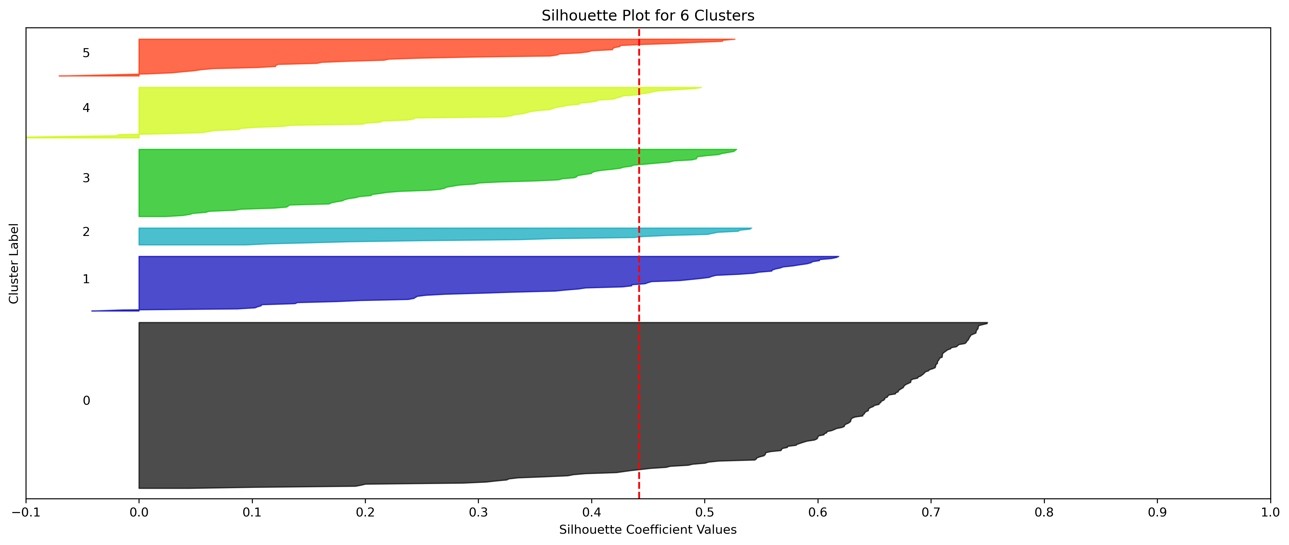
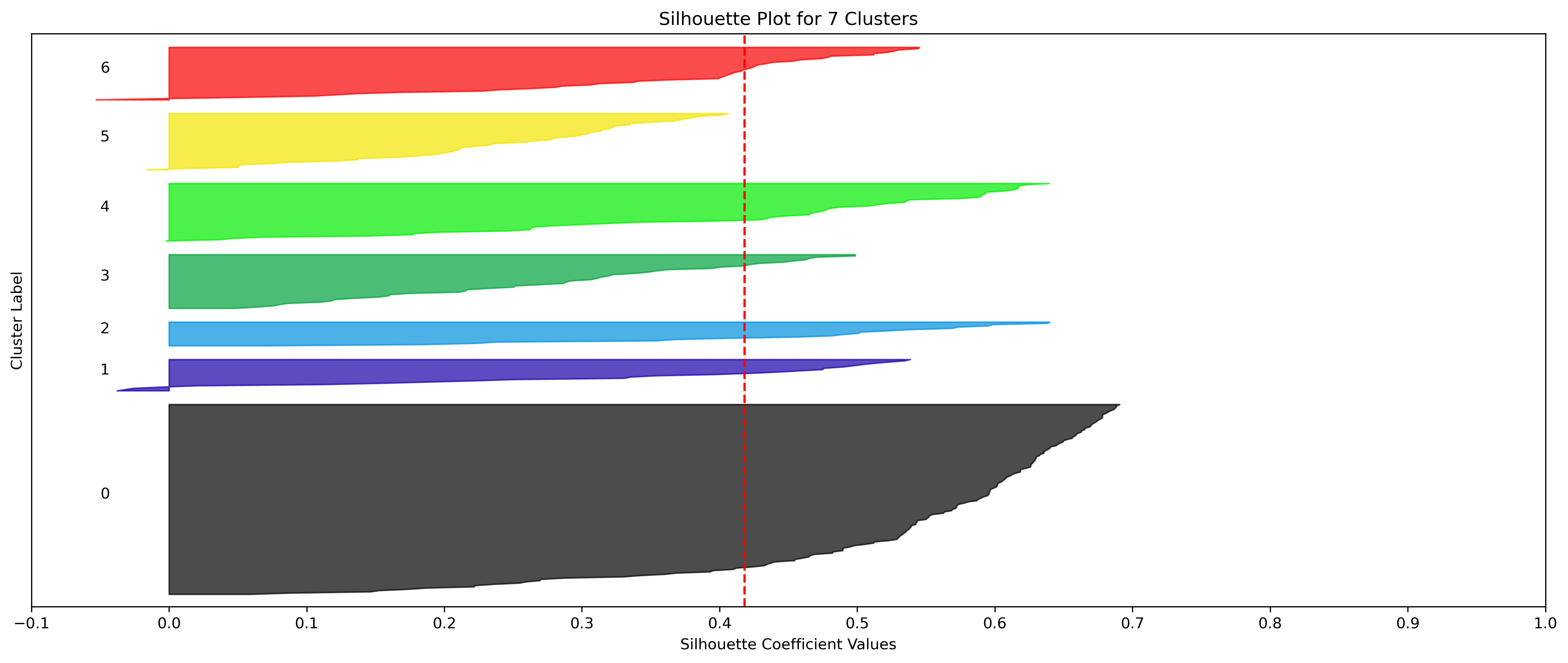
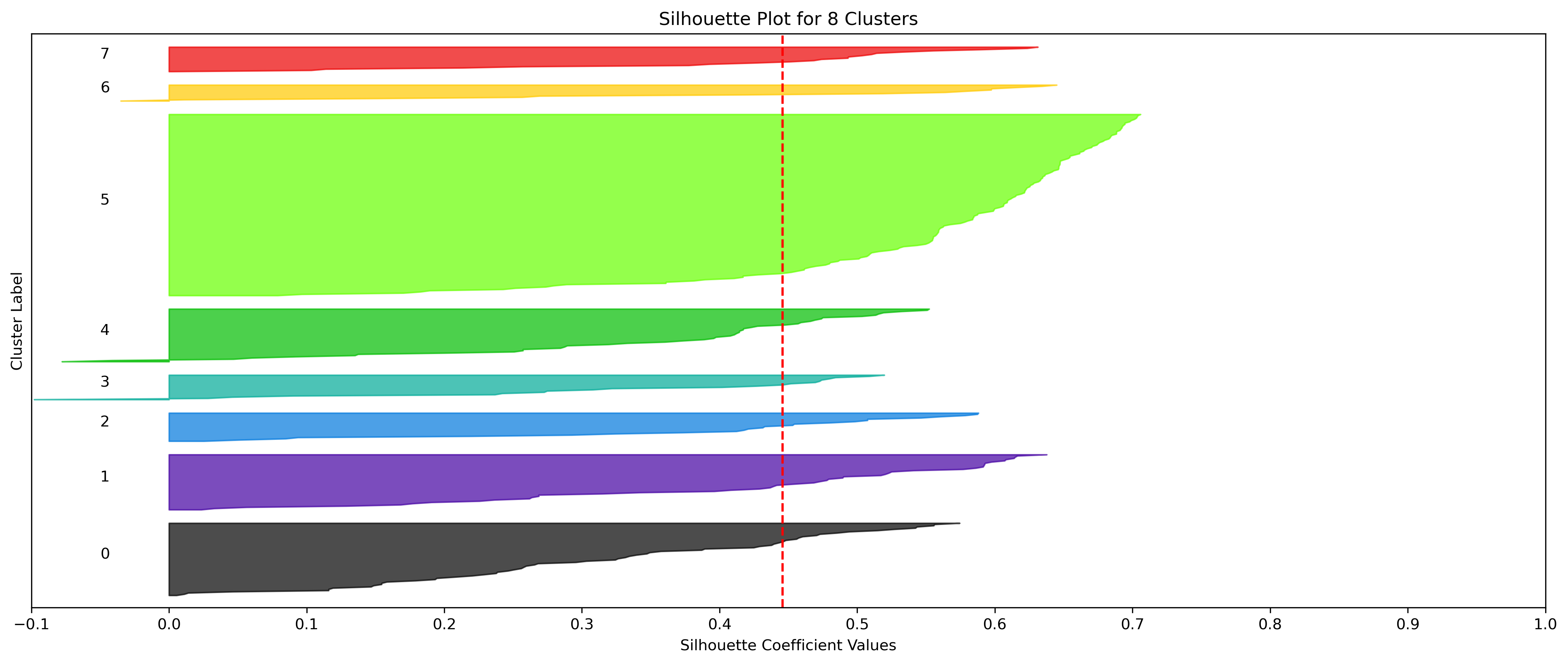
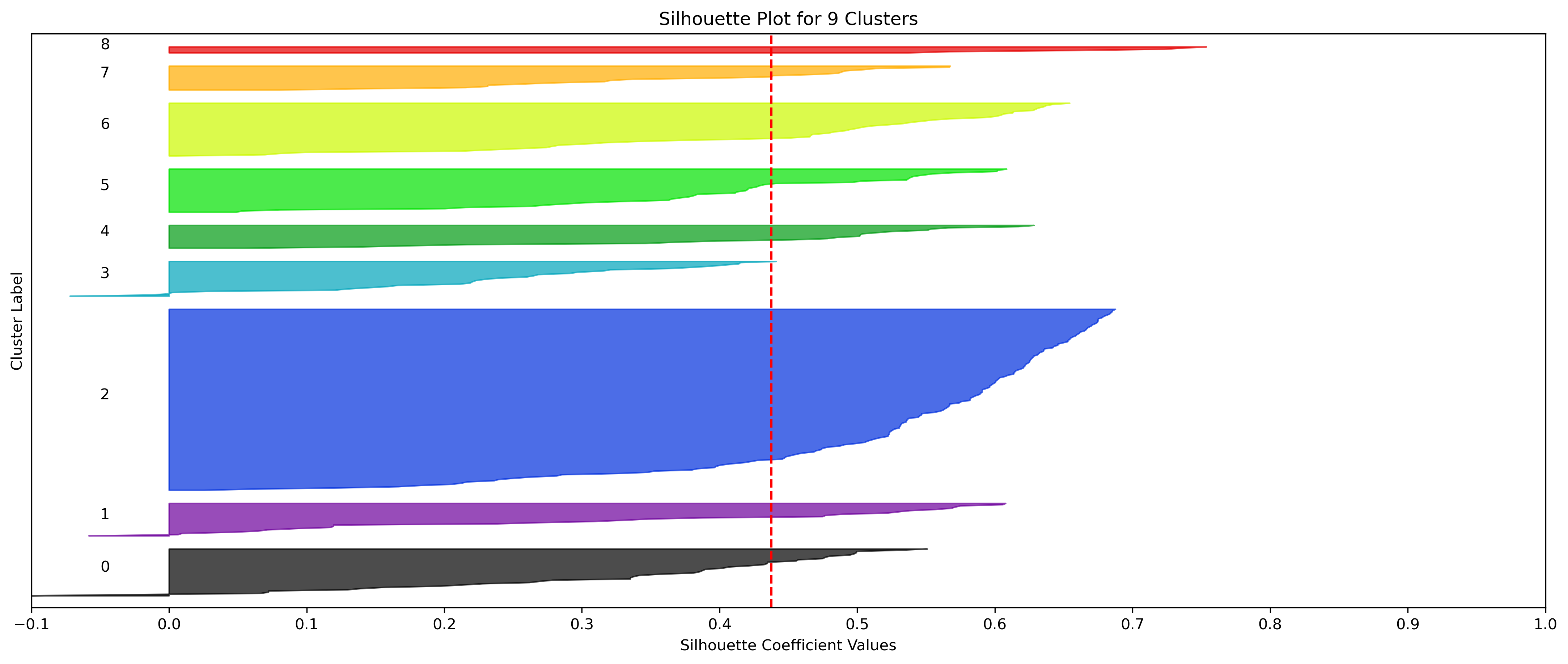
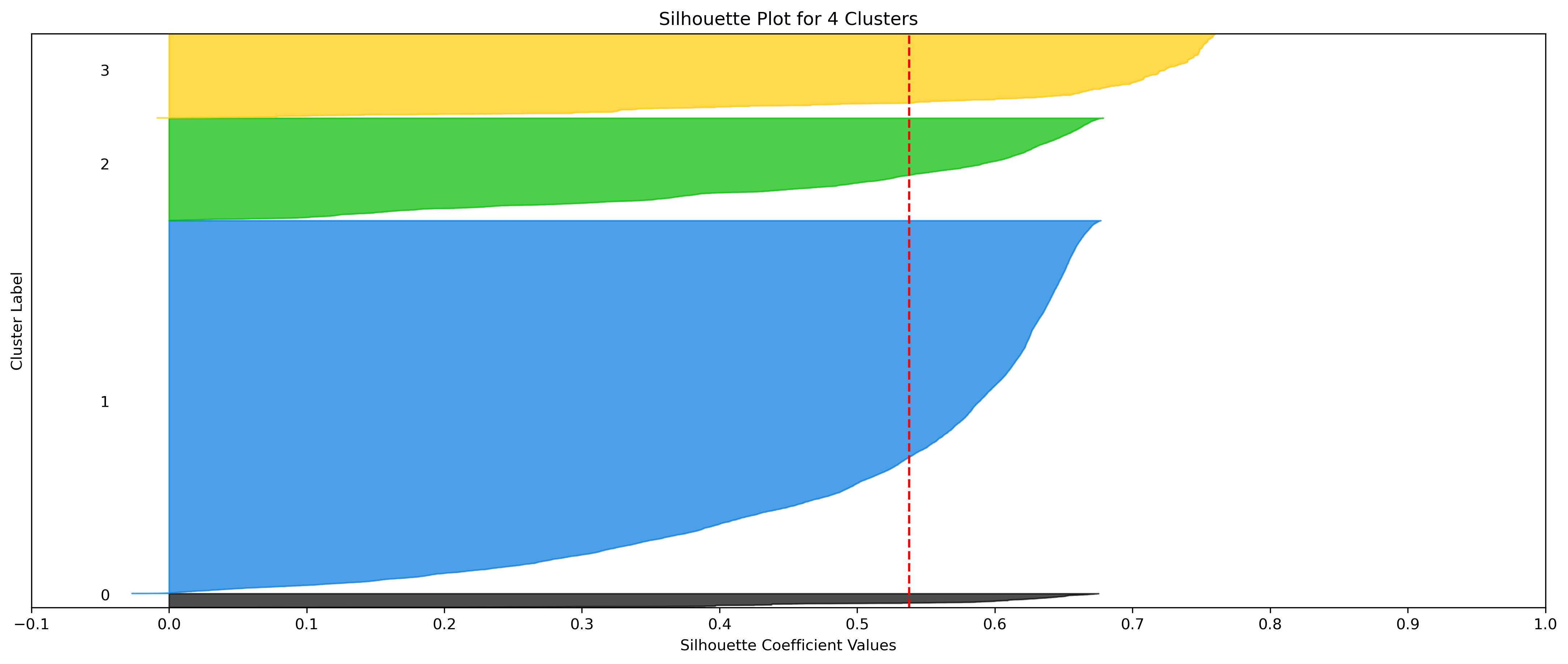
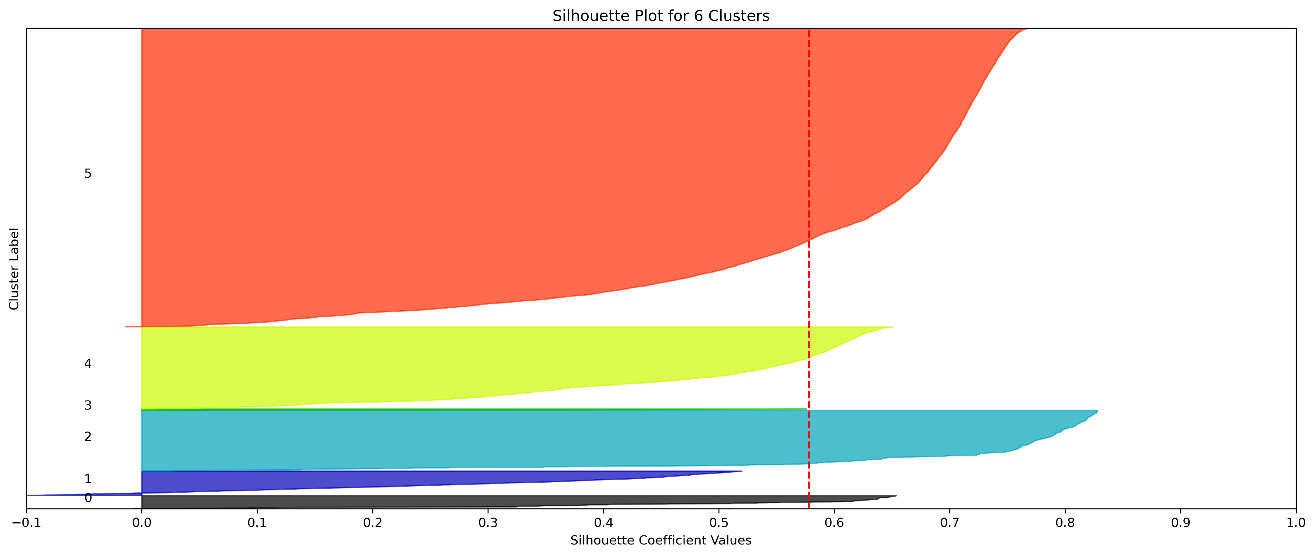
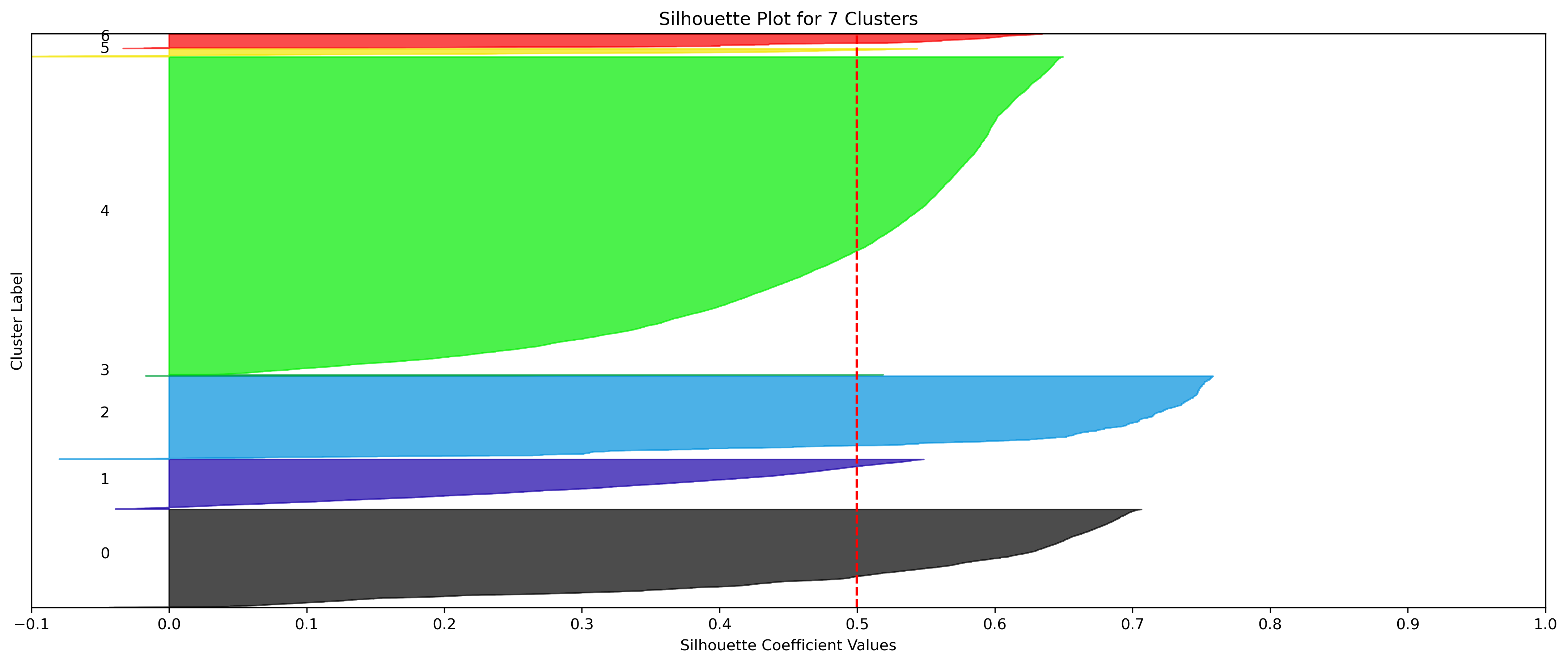
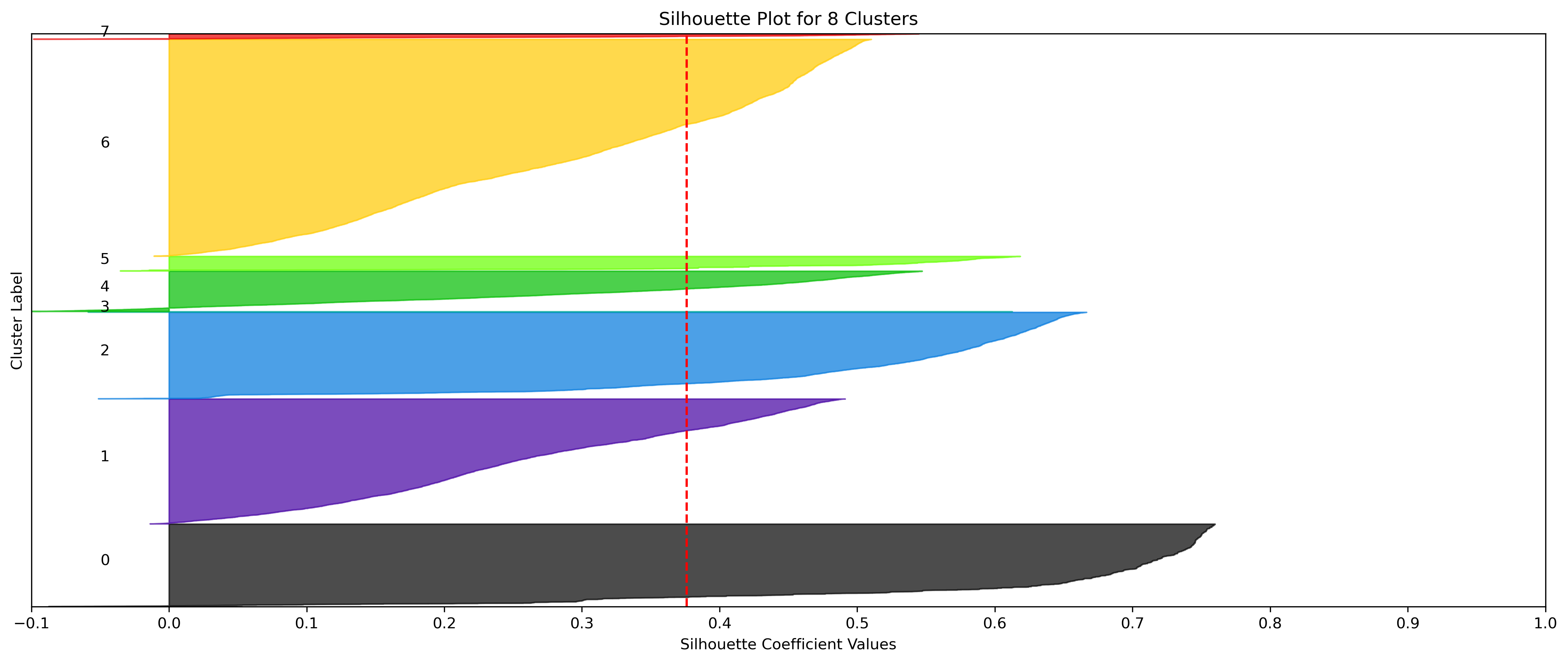
There are several different methods to choose an optimal number of clusters to use.
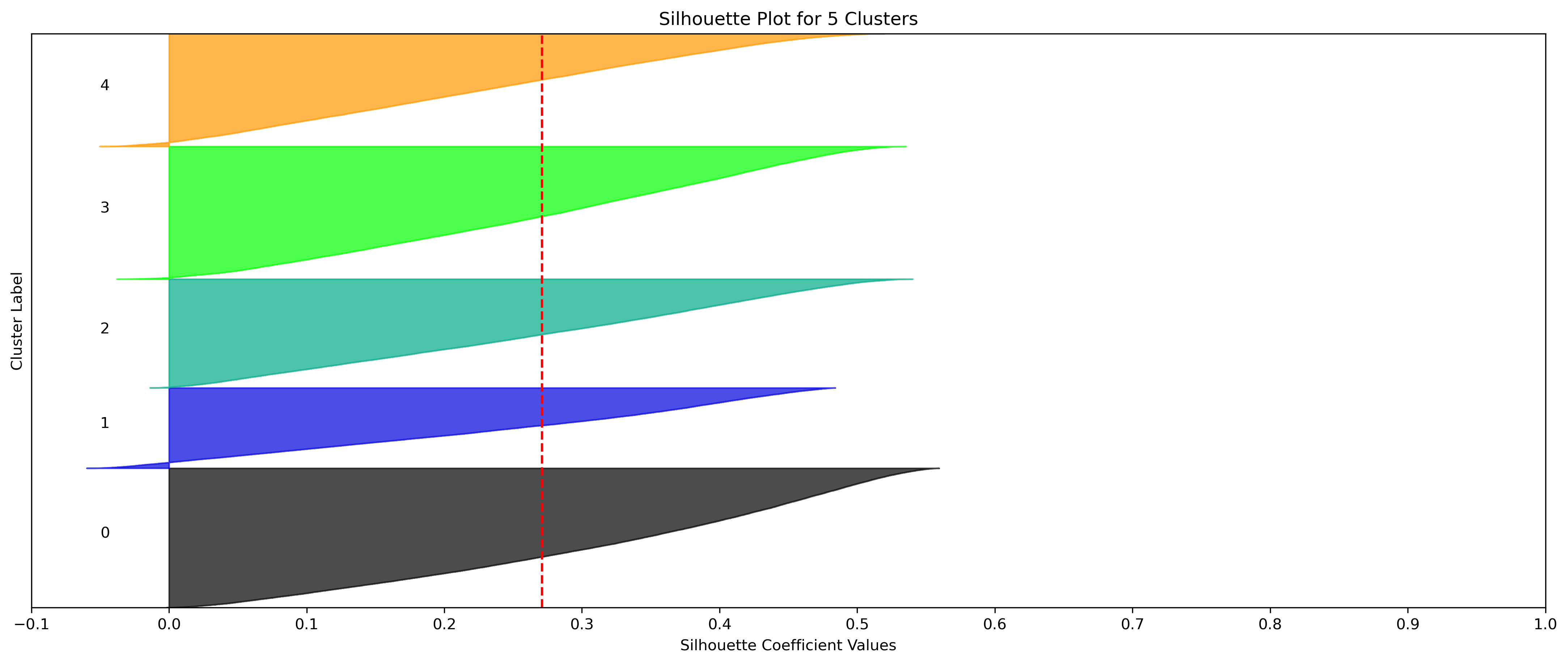
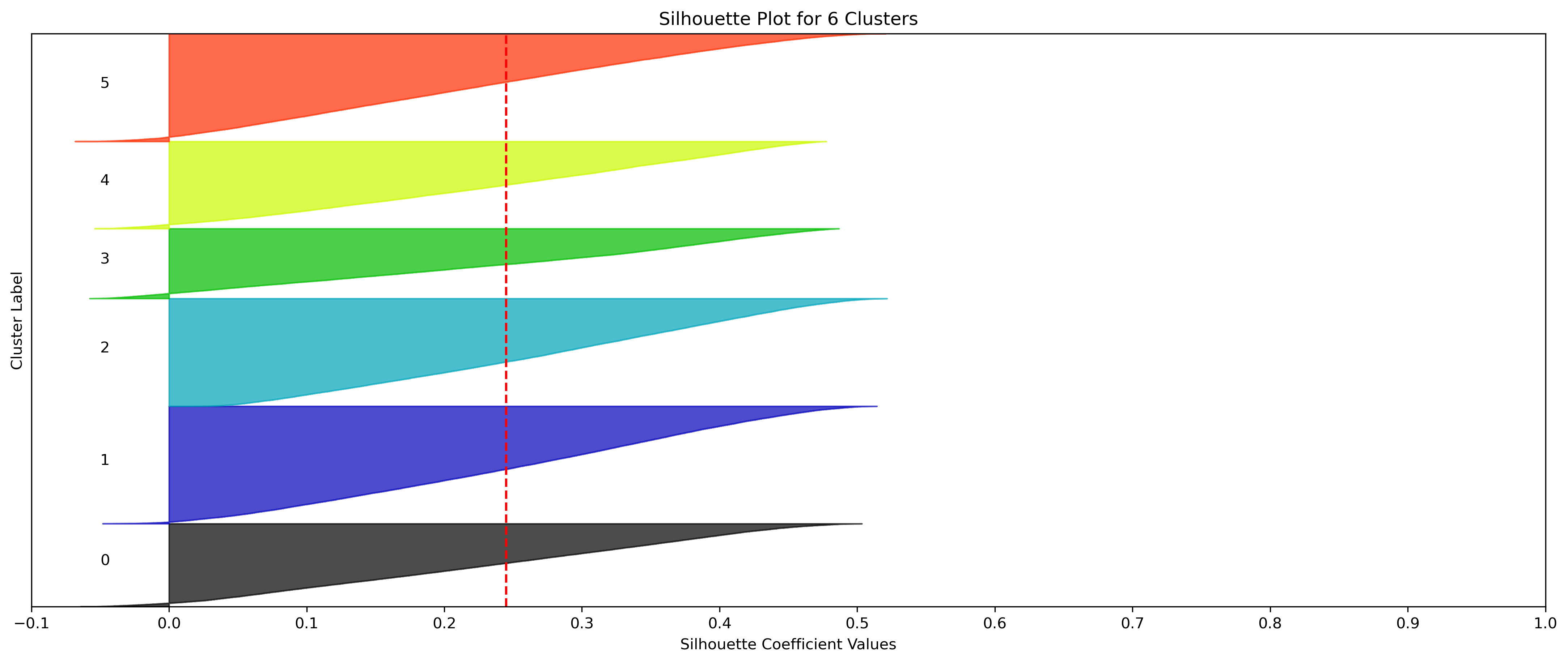
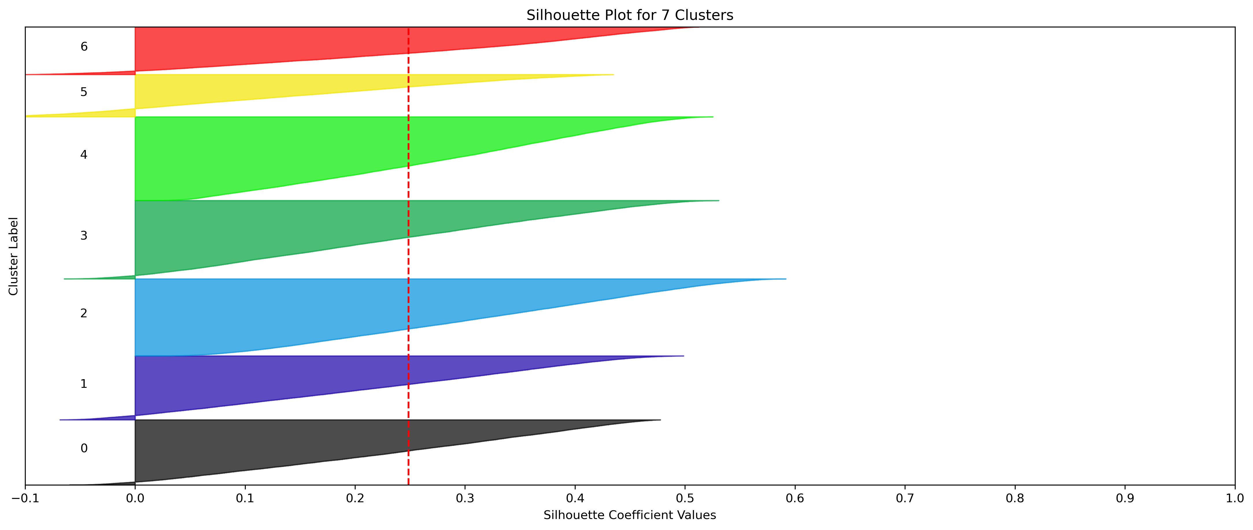
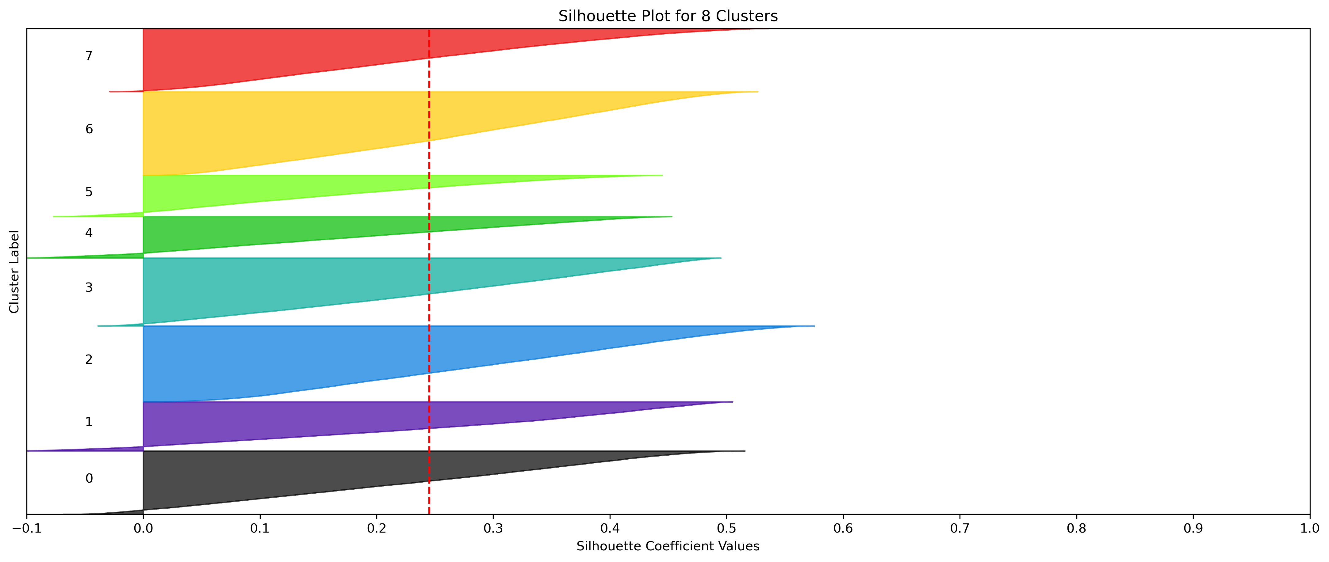
Using both the Silhouette Method and Elbow Method can help confirm this optimal amount.
This script can be found here, and
contains detailed documentation on these functions.
KMeans - Resorts
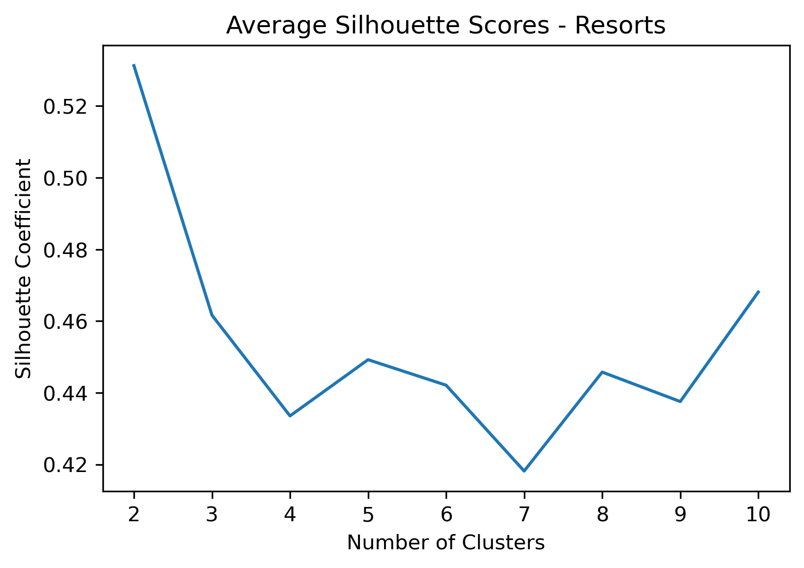
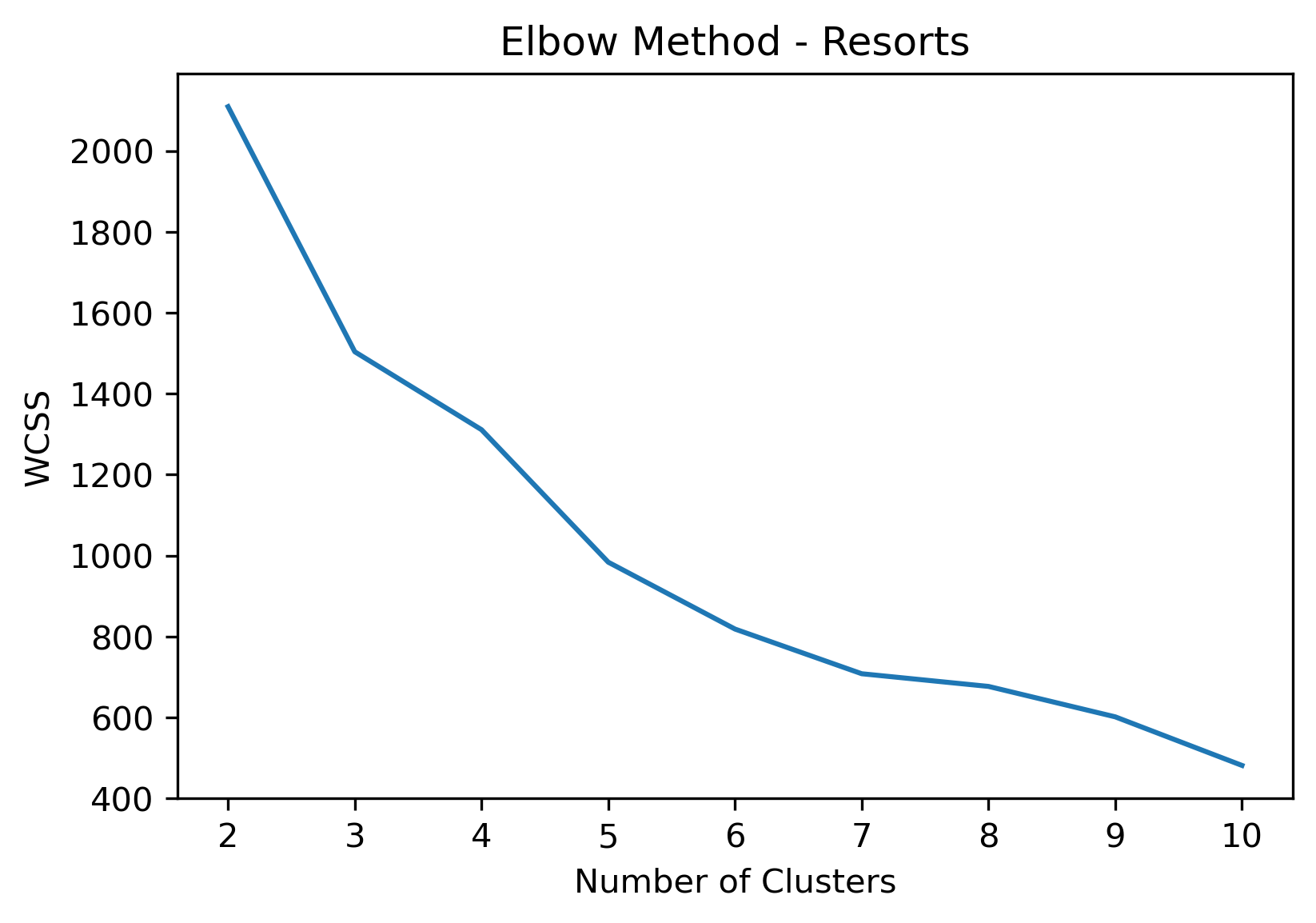
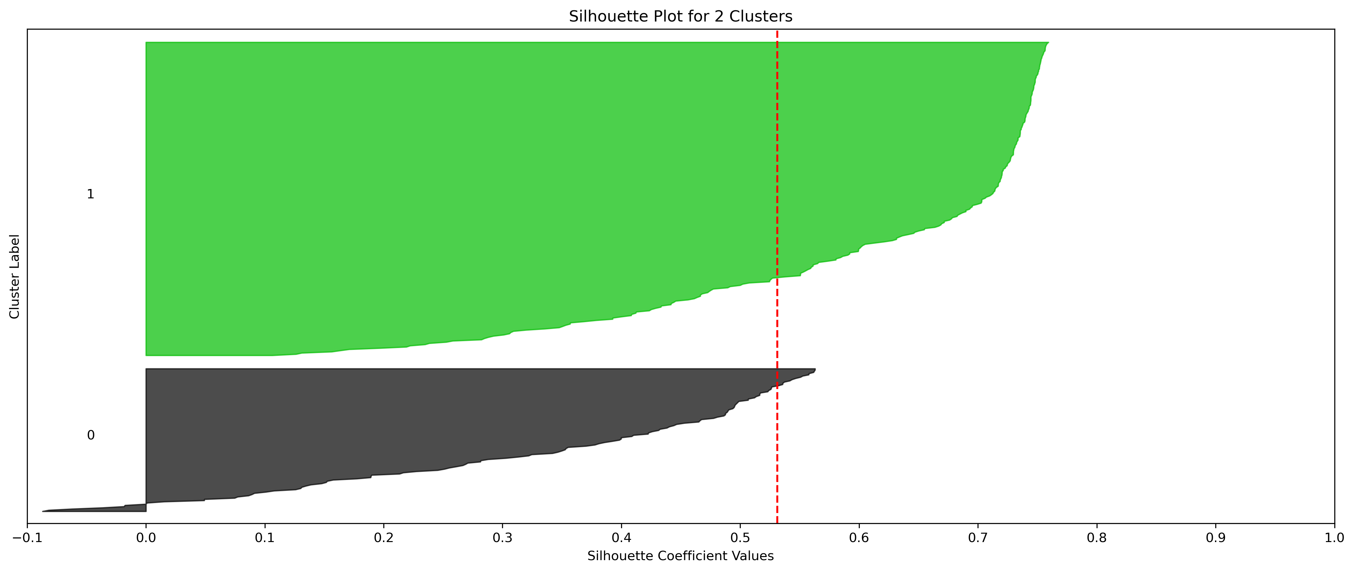
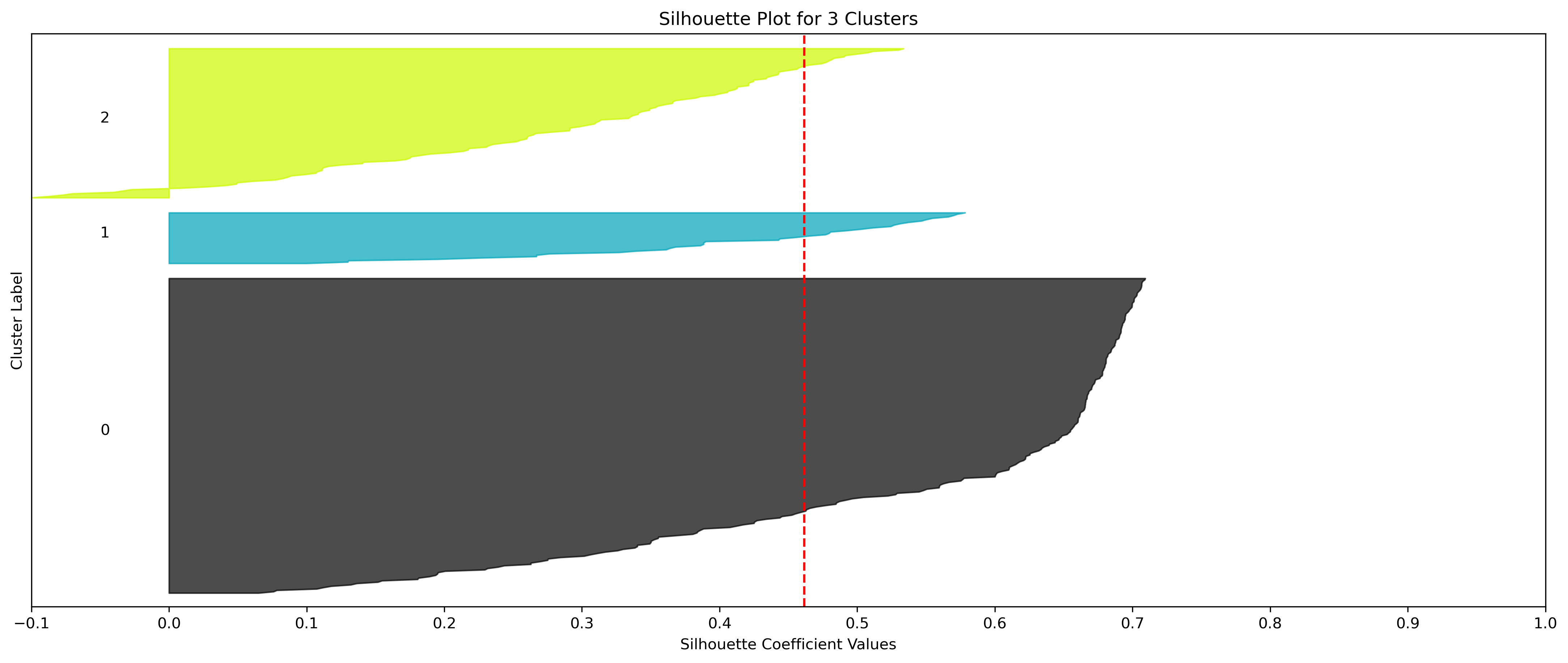
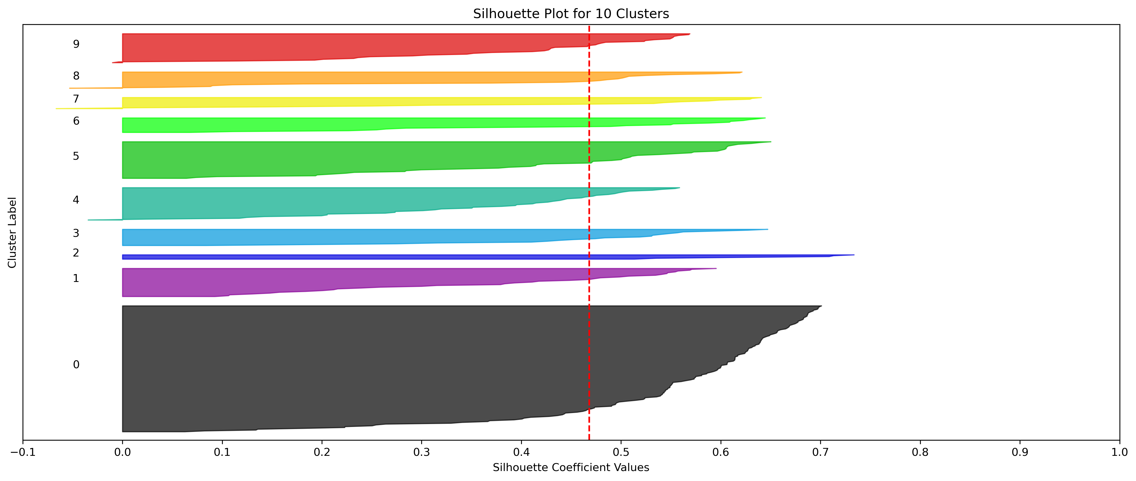
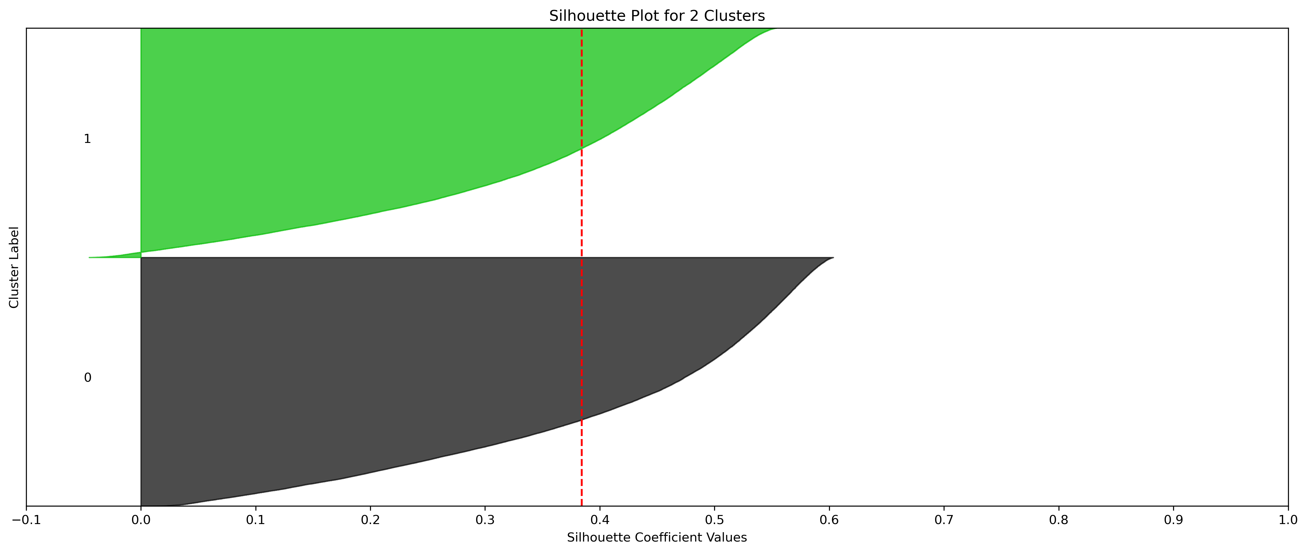
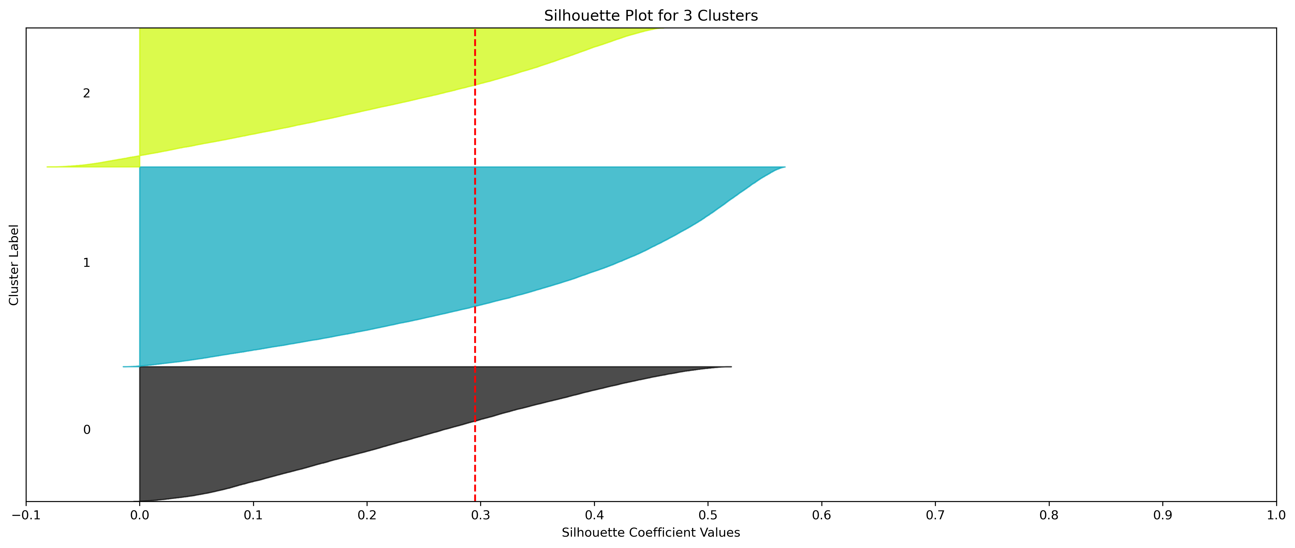
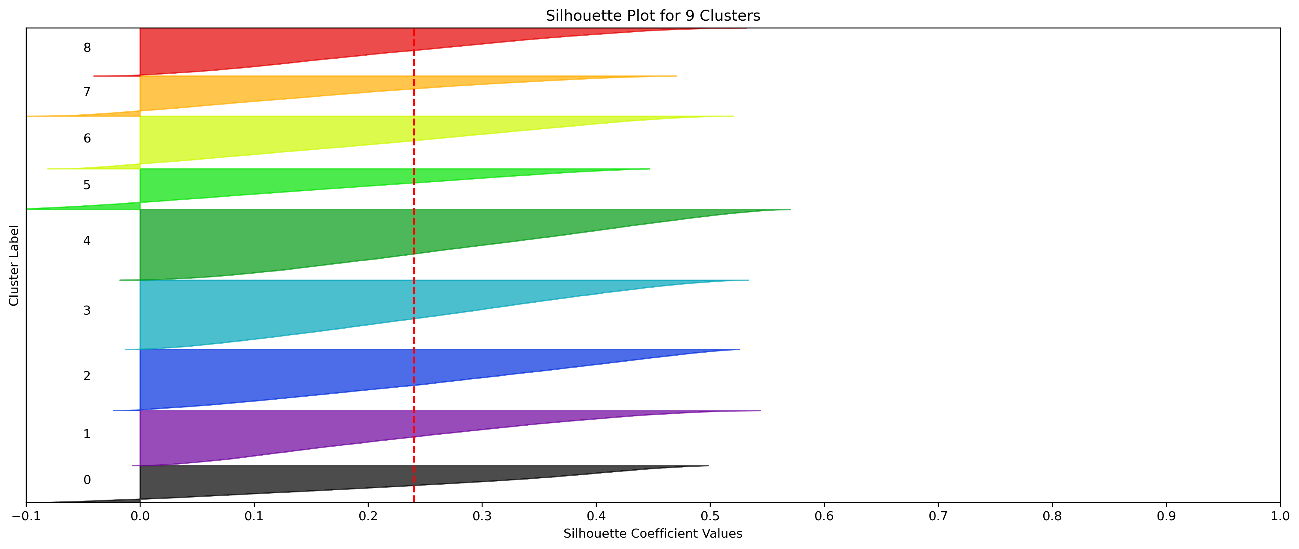
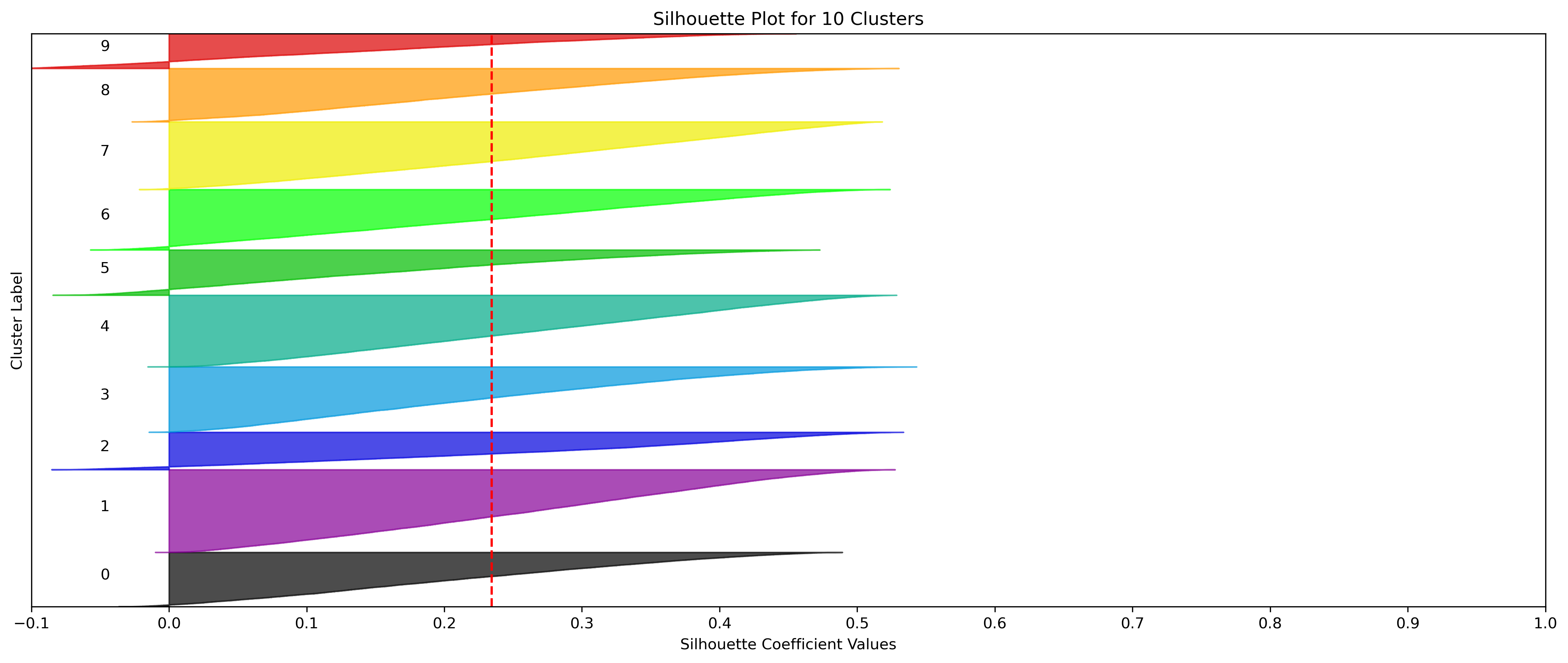
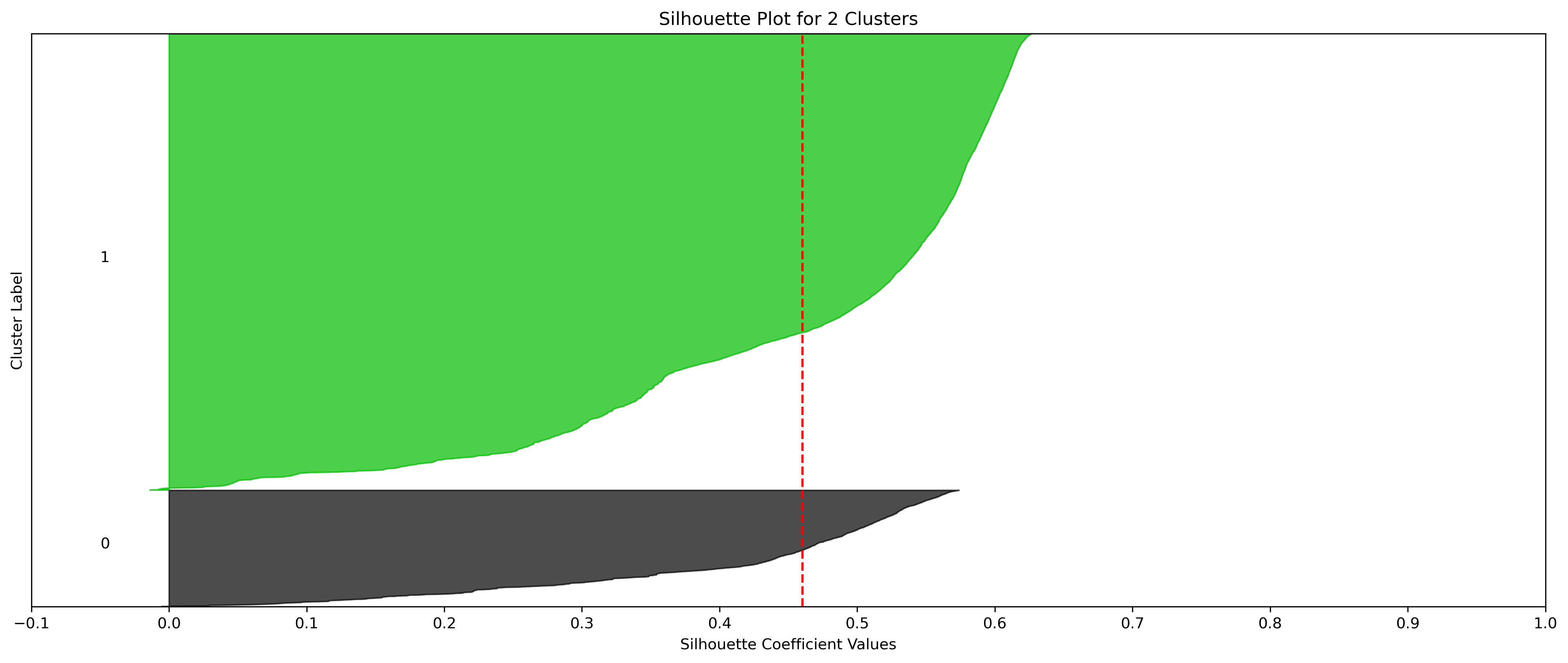
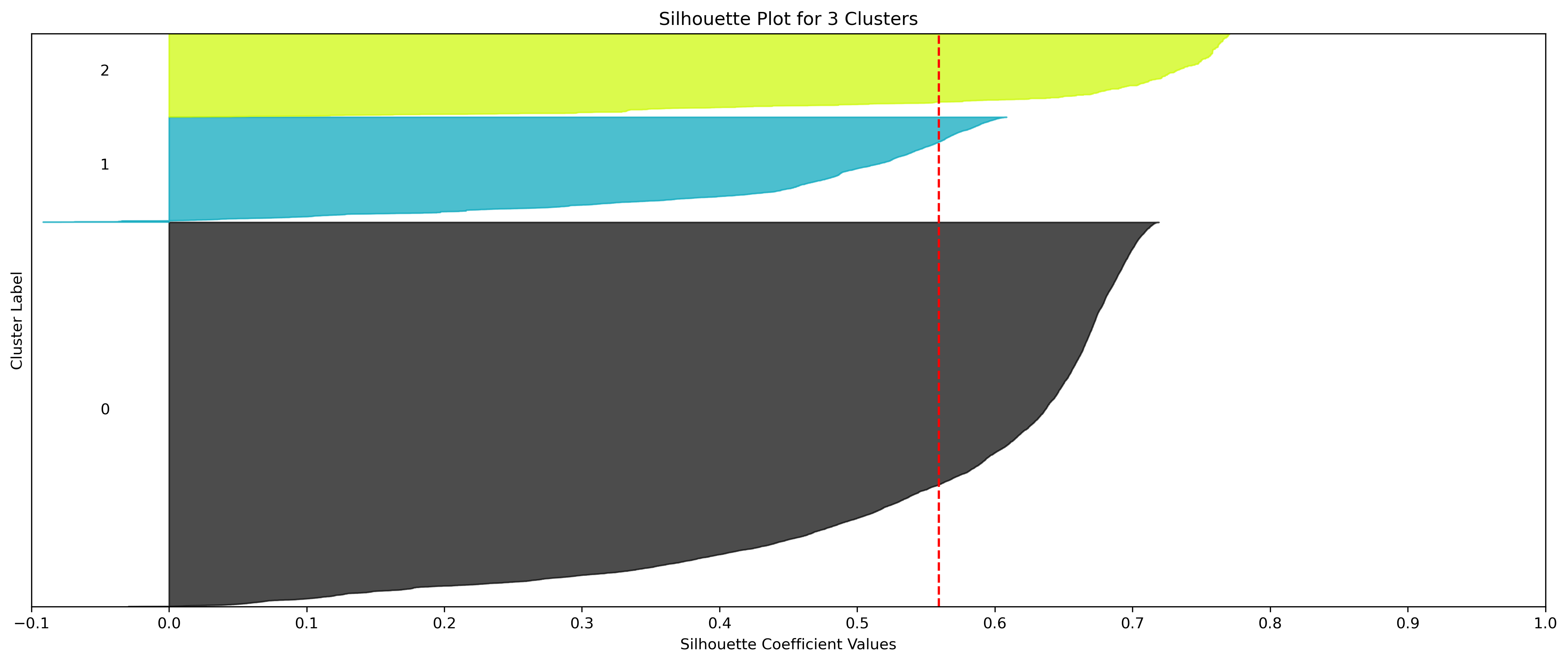
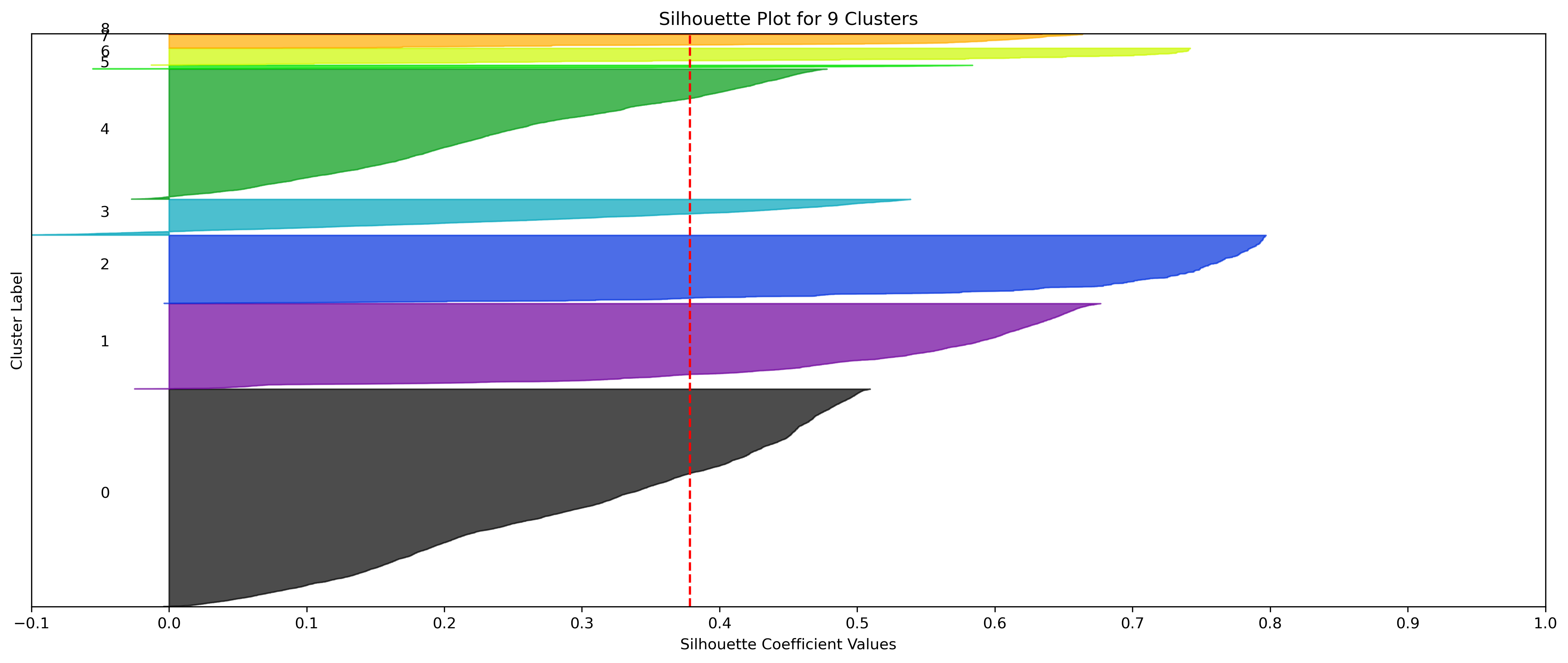
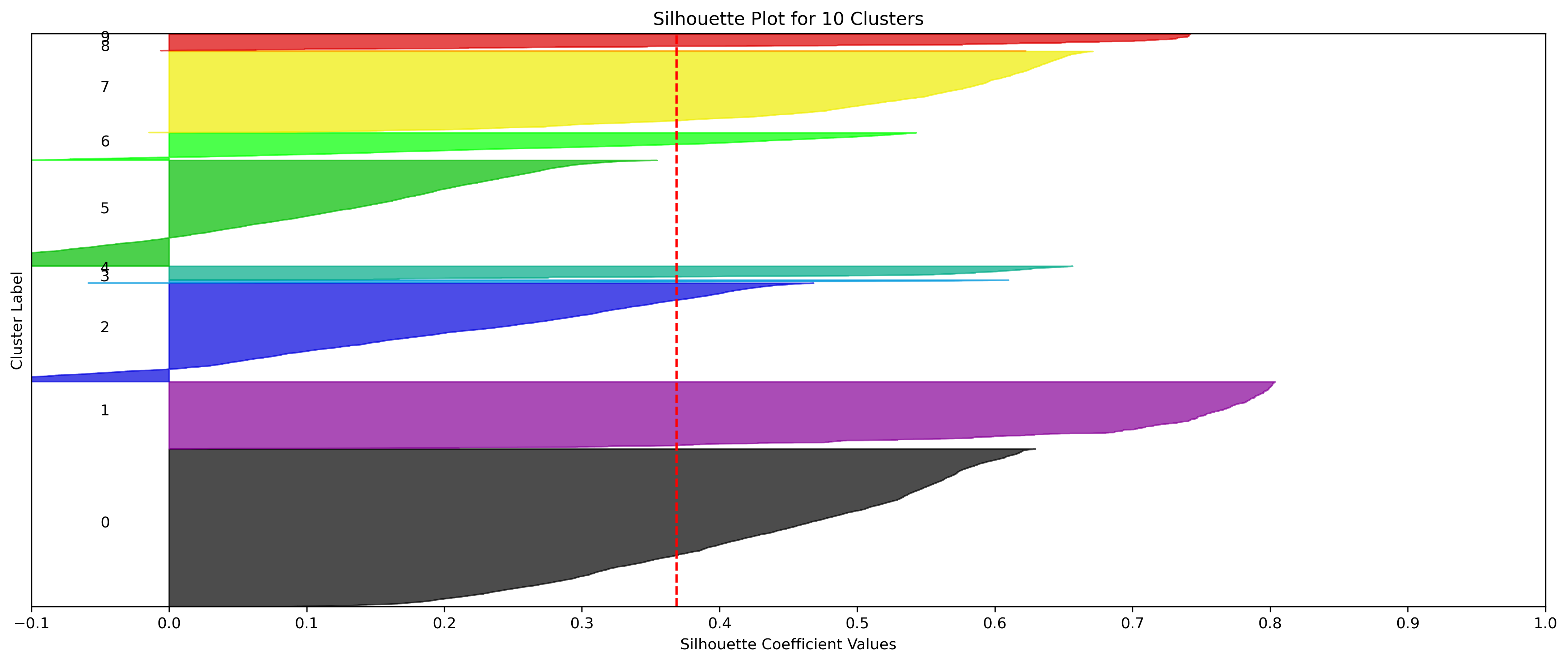
2, 3, and 10 clusters are decent choices for the optimal number of clusters for the Resorts data, with 3 showing strong potential to be the most optimal.
- k=2 Clusters
- Silhouette Method: 2 has the highest average silhouette score, with each cluster having datapoints with silhouette coefficients surpassing the silhouette average.
- Elbow Method: 2 isn't in a definitive elbow point, and likely wouldn't be recommended if only using this method.
- k=3 Clusters
- Silhouette Method: 3 has a relatively high average silhouette score, excluding 2, with each cluster having datapoints with silhouette coefficients surpassing the silhouette average.
- Elbow Method: 3 is a definitive elbow point, although it is a local elbow point with relatively high WCSS, it could be recommended using this method.
- k=10 Clusters
- Silhouette Method: 10 has a relatively high average silhouette score, excluding 2, with each cluster having datapoints with silhouette coefficients surpassing the silhouette average.
- Elbow Method: Although 10 is past the second elbow point, it does have the expectedly lowest WCSS. If there were more cluster groups considered, it could be possible that this is leading into another elbow point.
- Further Considerations
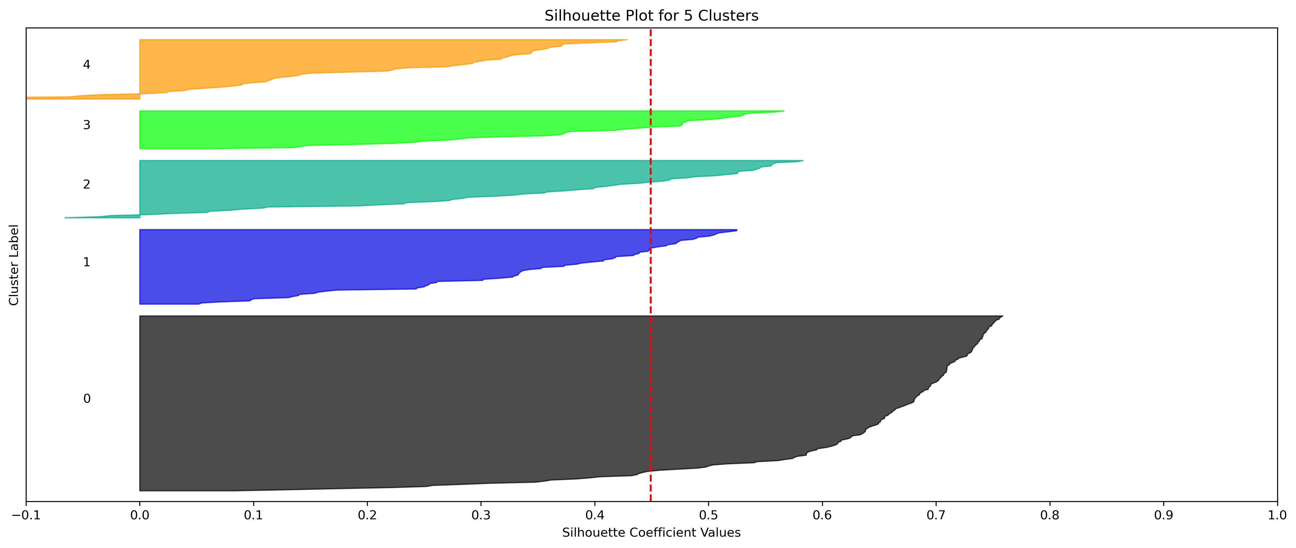
- k=5 Clusters has a decent average silhouette score, excluding 2, however one of the cluster's data has silhouette coefficients which do not meet the silhouette average score.
- k=5, 6, and 7 Clusters would likely be the strongest choices of clusters if strictly using the elbow method. However, as describe above, 5 clusters isn't a good choice due to the silhouette coefficients of one of its clusters, and 6 and 7 have the lowest silhouette averages of the tested clusters.
- k=8 Clusters would also be a decent option. This reduces computational overhead compared to k=10 Clusters, but the average silhouette score is lower than 2, 3, and 10.
KMeans - Weather
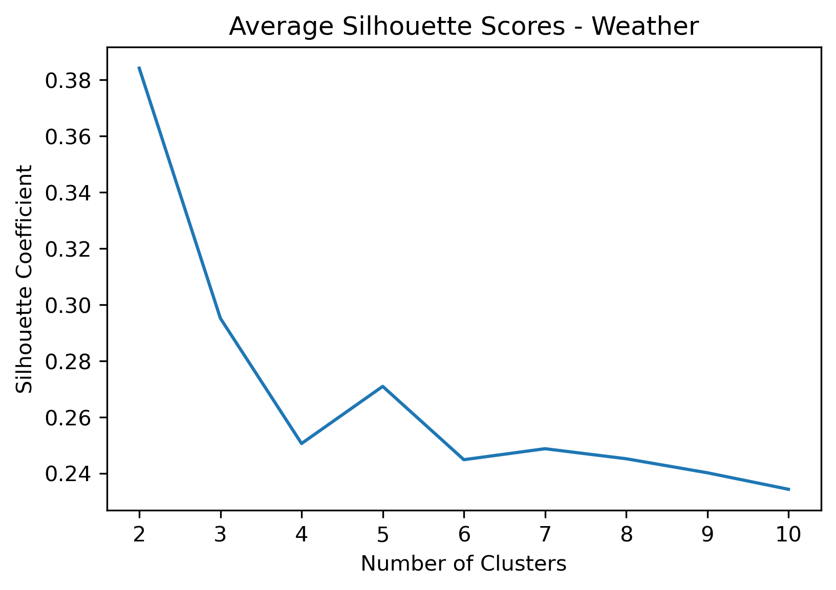
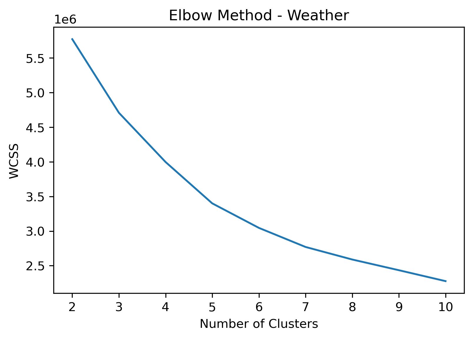
2, 3, and 5 clusters are decent choices for the optimal number of clusters for the Weather data, with 3 and 5 showing strong potential to be the most optimal.
- k=2 Clusters
- Silhouette Method: 2 has the highest average silhouette score, with each cluster having datapoints with silhouette coefficients surpassing the silhouette average.
- Elbow Method: 2 isn't in a definitive elbow point, and likely wouldn't be recommended if only using this method.
- k=3 Clusters
- Silhouette Method: 3 has a relatively high average silhouette score, excluding 2, with each cluster having datapoints with silhouette coefficients surpassing the silhouette average.
- Elbow Method: 3 is a definitive elbow point, although it is a local elbow point with relatively high WCSS, it could be recommended using this method.
- k=5 Clusters
- Silhouette Method: 5 has a relatively high average silhouette score, excluding 2, with each cluster having datapoints with silhouette coefficients surpassing the silhouette average.
- Elbow Method: 5 is a definitive elbow point, and would likely be the suggested number of clusters if strictly using this method.
- Further Considerations
- k=2, 3, and 5 have the highest average silhouette scores.
- All clusters tested have datapoints in which every cluster has datapoints with silhouette coefficents surpassing the average silhouette score.
- All clusters tested have a relatively uniform distribution of datapoints across clusters, indicated by the size of the silhouette coefficients.
- Although the silhouette averages and coefficients indicate decent choices for number of clusters, the scores for k=6, 8, 9, and 10 have relatively low average silhouette scores, which taper down even moreso after 7.
- k=7 Clusters could be another choice, even being an elbow point in the Elbow Chart. However, the chosen 3 cluster numbers have better relative average silhouette scores.
KMeans - Google
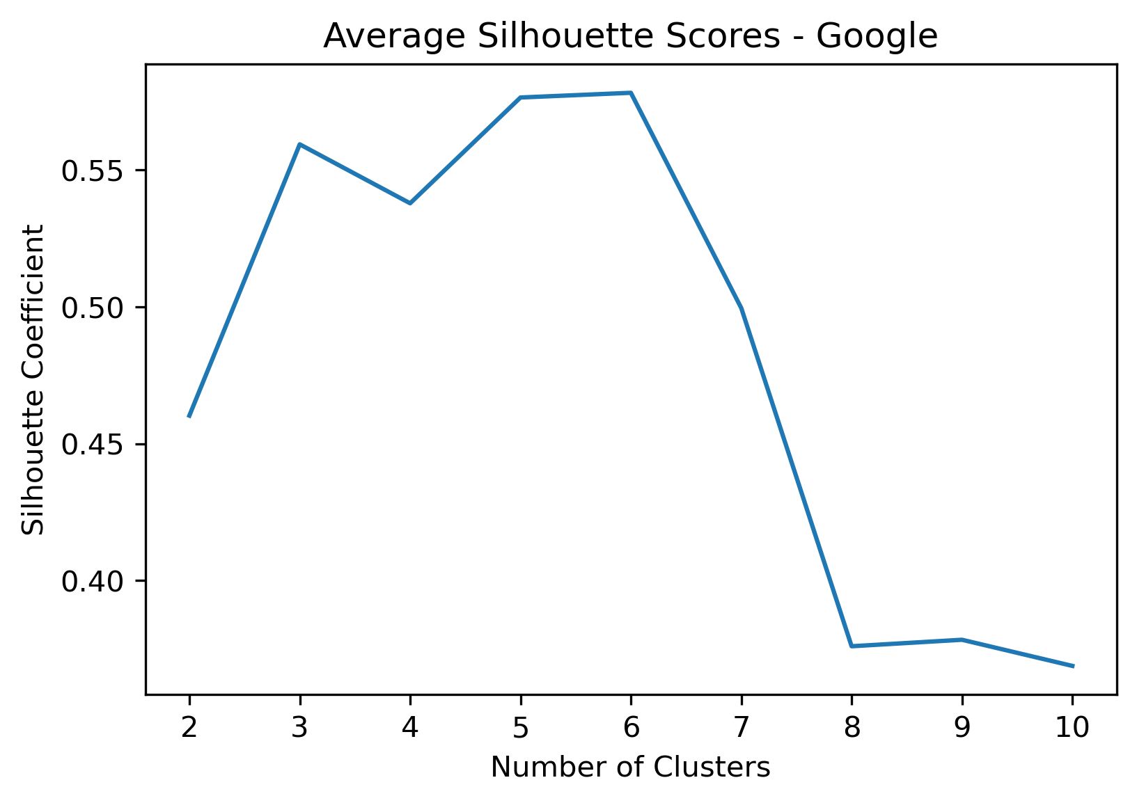
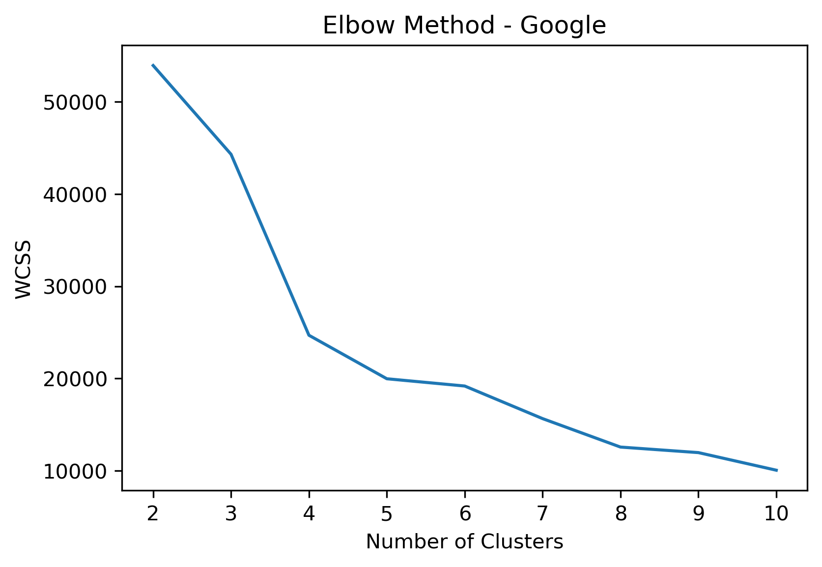
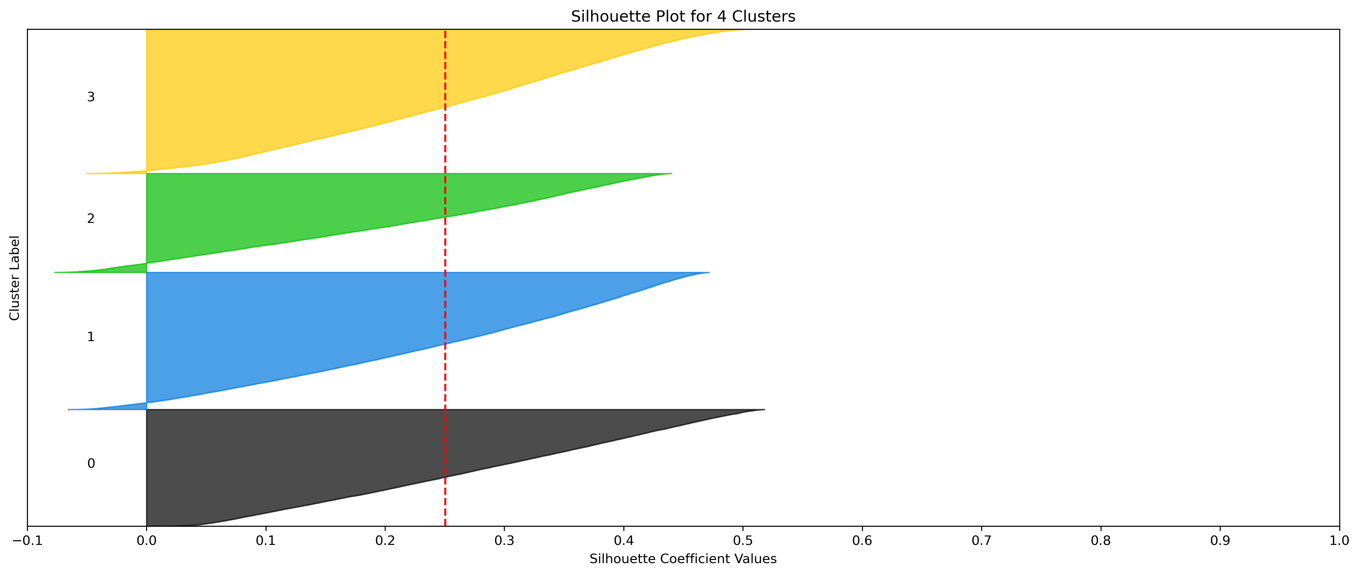
4, 5 and 6 clusters are decent choices for the optimal number of clusters for the Google data, with 5 and 6 showing strong potential to be the most optimal.
- k=4 Clusters
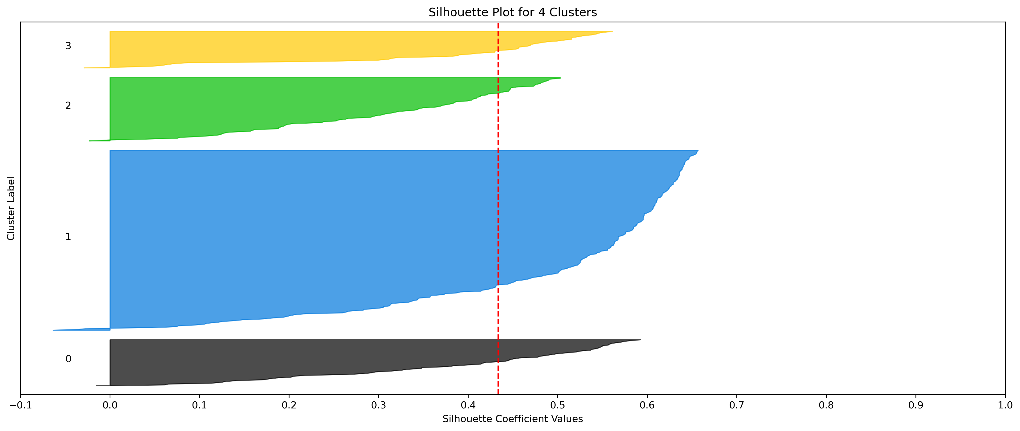
- Silhouette Method: Although 3 clusters has a higher average silhouette score, 4 is still among the highest average silhouette scores. Each cluster has datapoints with silhouette coefficients surpassing the silhouette average.
- Elbow Method: Cluster choices of 4, 5, and 6 are optimal choices according to this method.
- k=5 Clusters
- Silhouette Method: 5 clusters has the second highest average silhouette scores. One of the clusters with a small proportion of datapoints doesn't have silhouette coefficients which surpass the silhouette average, but that could be due to the proportion of data clustered into that group on an otherwise clustering with a high average.
- Elbow Method: Cluster choices of 4, 5, and 6 are optimal choices according to this method.
- k=6 Clusters
- Silhouette Method: 6 clusters has the highest average silhouette scores. One of the clusters with a small proportion of datapoints doesn't have silhouette coefficients which surpass the silhouette average, but that could be due to the proportion of data clustered into that group on an otherwise clustering with a high average.
- Elbow Method: Cluster choices of 4, 5, and 6 are optimal choices according to this method.
- Further Considerations
- Although k=3 Clusters has the third highest average silhouette score, using k=4 Clusters (fourth highest average silhouette score) was further validated via the elbow method.
- All clusters tested have datapoints in which every cluster has datapoints with silhouette coefficents surpassing the average silhouette score.
- All clusters tested have a relatively uniform distribution of datapoints across clusters, indicated by the size of the silhouette coefficients.
- Although the silhouette averages and coefficients indicate decent choices for number of clusters, the scores for k=8, 9, and 10 have significantly lower average silhouette scores than the rest of the cluster choices. Additionally, they aren't quite supported by the elbow method.
KMeans Visualization - Resorts
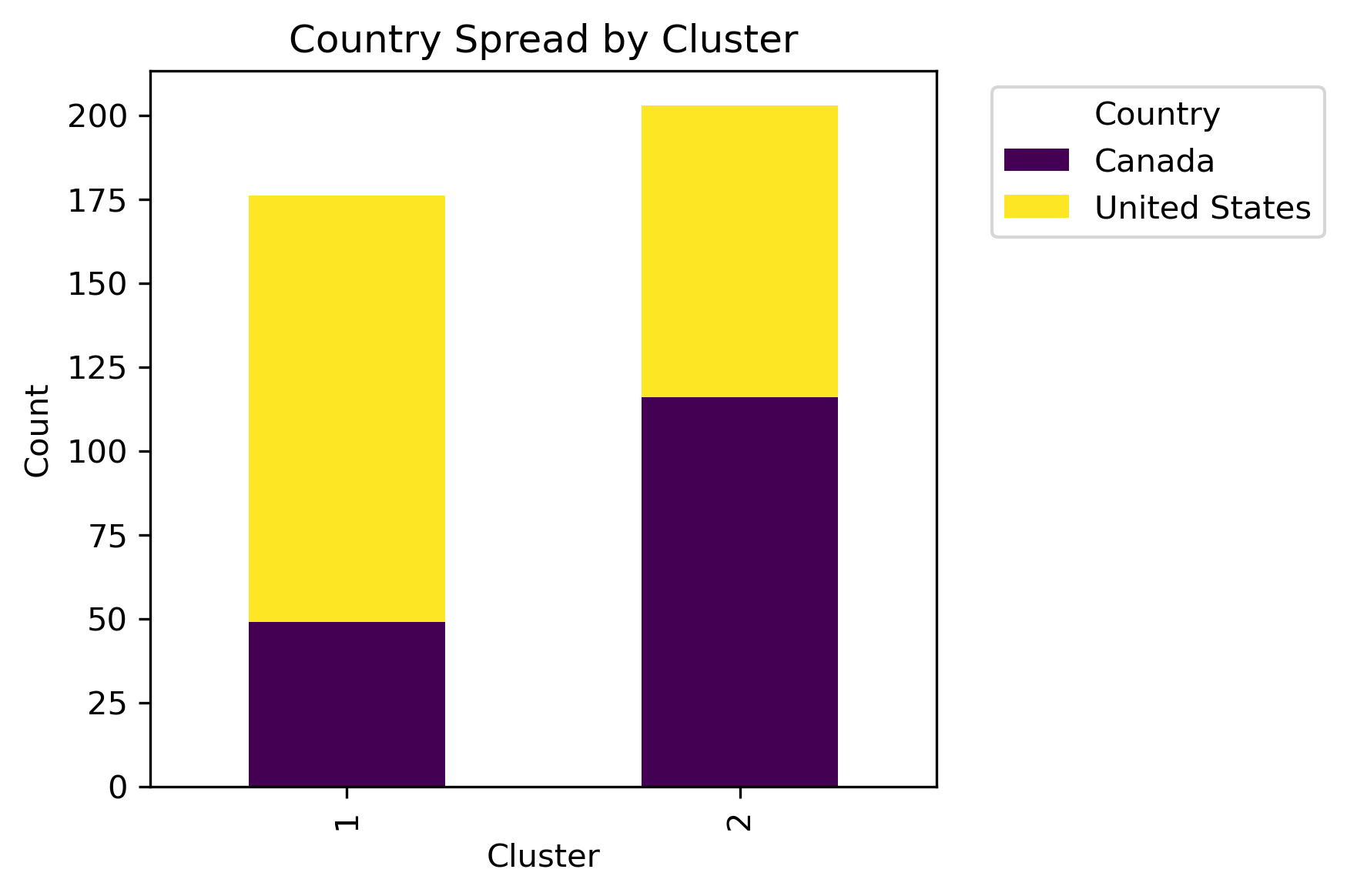
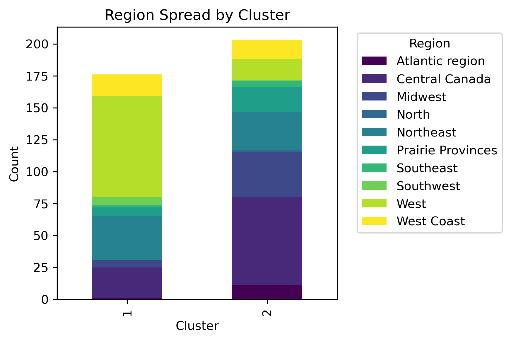
For the Resorts data, clustering was performed for the following combinations of clusters and labels:
- Clusters
- 2 Clusters
- 3 Clusters
- 10 Clusters
- Labels
- Country: United States and Canada
- Pass: type of ski pass associated with the businesses near a given ski resort
- Region: 10 different spatial boundaries across North America
KMeans Visualization - Weather
For the Weather data, clustering was performed for the following combinations of clusters and labels:
- Clusters
- 2 Clusters
- 3 Clusters
- 5 Clusters
- Labels
- Icon: weather type for a given time period returned by the weather API
- Month: illustrate how the clusters evolve over months via average monthly aggregation
For each combination, the legend features are toggleable.
KMeans Visualization - Google
For the Google data, clustering was performed for the following combinations of clusters and labels:
- Clusters
- 4 Clusters
- 5 Clusters
- 6 Clusters
- Labels
- Call Category: the business type that was passed to the Google Places API
- Country: United States and Canada
- Pass: type of ski pass associated with the businesses near a given ski resort
- Region: 10 different spatial boundaries across North America
For each combination, the legend features are toggleable.
KMeans Clustering Results and Discussion
Hierarchical Clustering
Hierarchical Clustering determines cluster assignments by building a hierarchy, either bottom-up (agglomerative) or top-down (divisive), and produces a tree-based hierarchy of points called a dendrogram. There are two main types of hierarchical clustering:
-
Agglomerative (agnes)
- bottom-up
- starts with the points as individual clusters (i.e. each observation is initially considered as single-element cluster)
- at each step, merge the closest pair of clusters until only one cluster (or specified k clusters) left
-
Divisive (diana)
- top-down
- starts with one, all-inclusive clsuter (i.e. every observation in a single cluster)
- at each step, split a cluster until each clsuter contains a point (or specified k clusters) left
The common machine learning libraries which allow for hierarchical clustering mostly use agglomerative clustering (bottom-up). Scikit-Learn has a module for this,
sklearn.cluster.AgglomerativeClustering, however, this mainly relies on
a specified number of clusters input. A more common approach in analysis of this sort is to use scip.cluster.hierarchy with dendrogram and linkage. This particular analysis will feature SciPy's libraries and modules.
Functions were created and then applied to create and analyze agglomerative dendrograms.
The functions script can be found here, and contains detailed documentation.
The applications of the functions can be found here.
Note that the same three-dimensional PCA space projected data on the three main datasets were used again for hierarchical clustering, however the Resorts data provided the best results.
Hierarchical Clustering - Resorts
The following process of analysis was applied to the Resorts data:
- Run three-dimensional PCA on the data.
- Create Linkage Matrix using the reduced dataset using the Ward's method.
- Create dendrogram with parameters which essentially shows a complete bottom-up approach.
- Tune parameters to investigate different tree clusters.
- Expand leaves.
Complete Hierarchical Tree
The complete bottom-up visualization for the Resorts data:
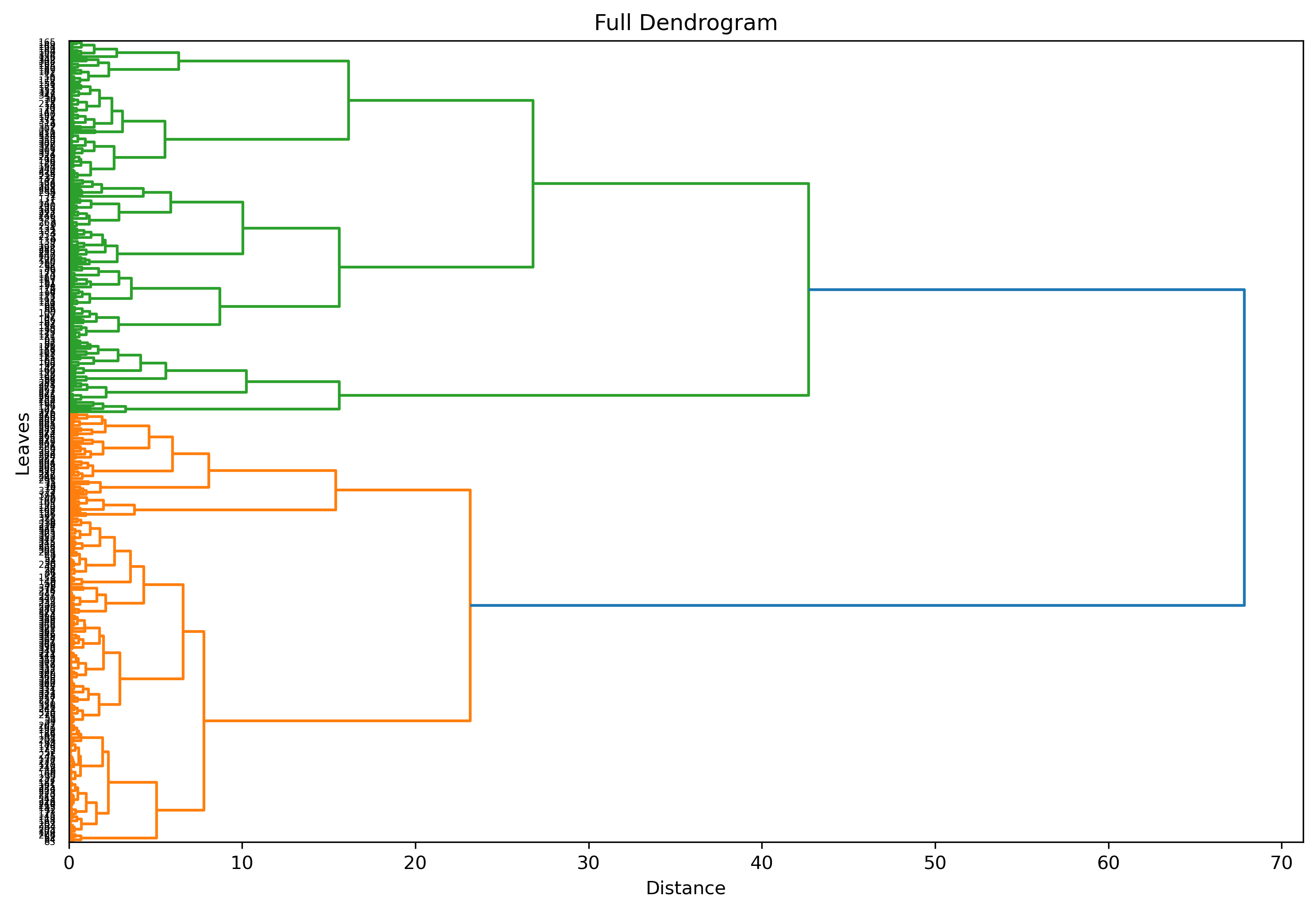
There are a few things to note about this image:
- The parameters show 2 clear clusters (green and orange) under the final child cluster (blue) which contains all observations.
- The tree has increasing splits at the beginning, stemming from initial observations as their own clusters.
- The initial observation nodes are difficult to interpret. In fact, the dendrogram doesn't give much interpretation value in its current state.
Truncated to Level 3 - Default Threshold
Truncating the dendrogram to level 3 will yield something more reasonable:
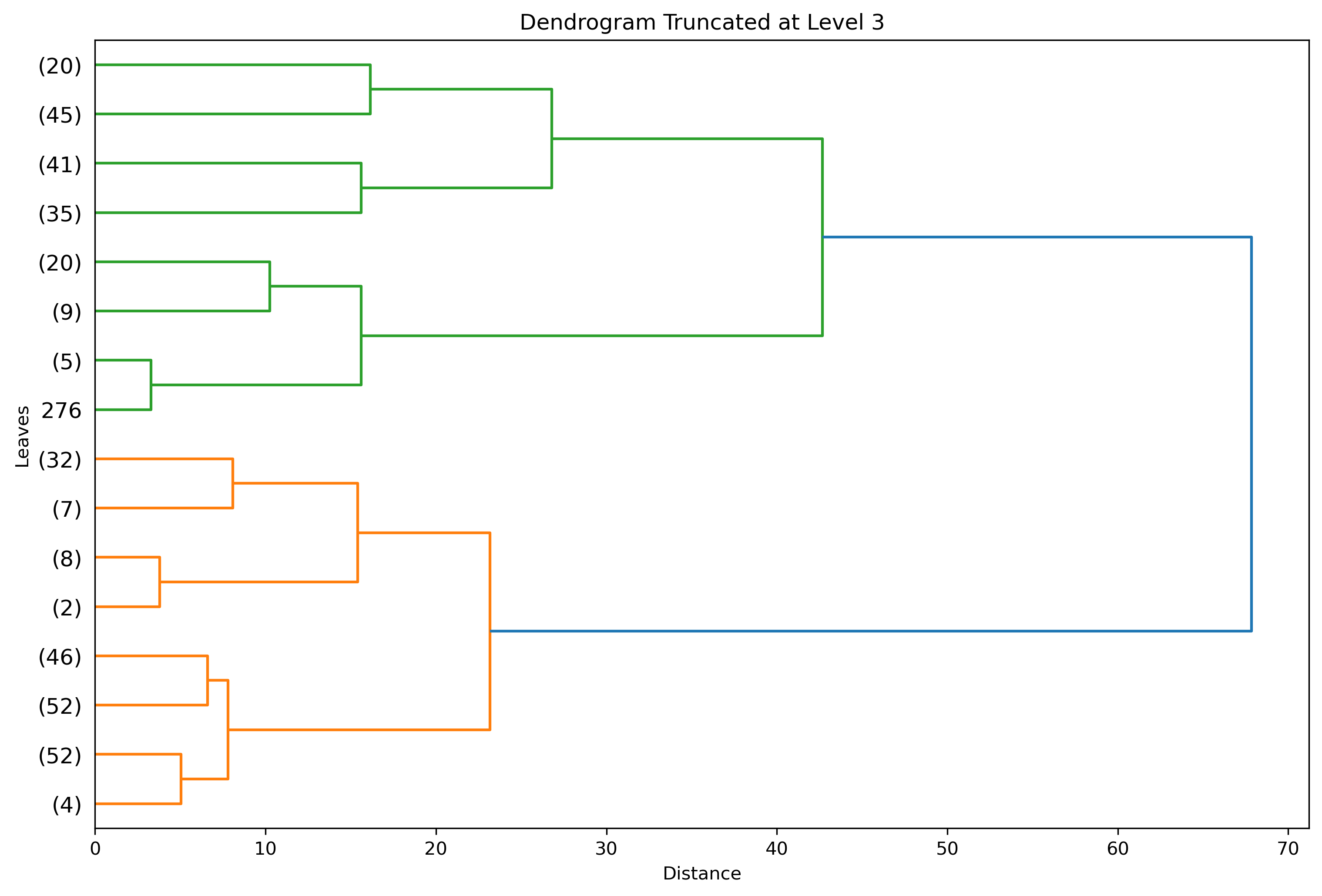
There are a few things to note about this image:
- The parameters show 2 clear clusters (green and orange) under the final child cluster (blue) which contains all observations.
- There is a similar result to the full dendrogram, however this version is more interpretable. At the very least, the leaves (final nodes) are readable.
- Leaves with
(number)indicatenumberof original observations under that leaf. - Leaves with
numberindicate theindexof a single original observation ending in that branch. If labels are provided, leaves with this format would produce a label. - Truncating at level 3 results in 3 tree layers underneath the final child cluster.
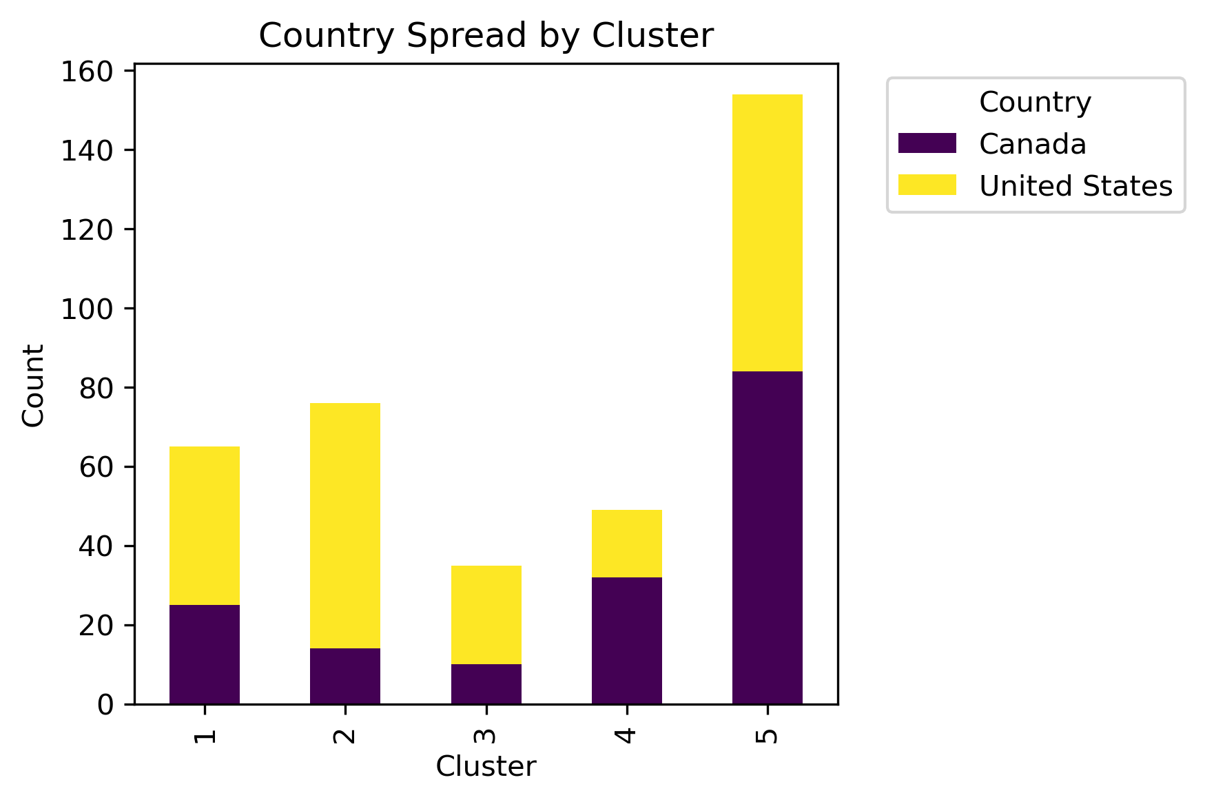
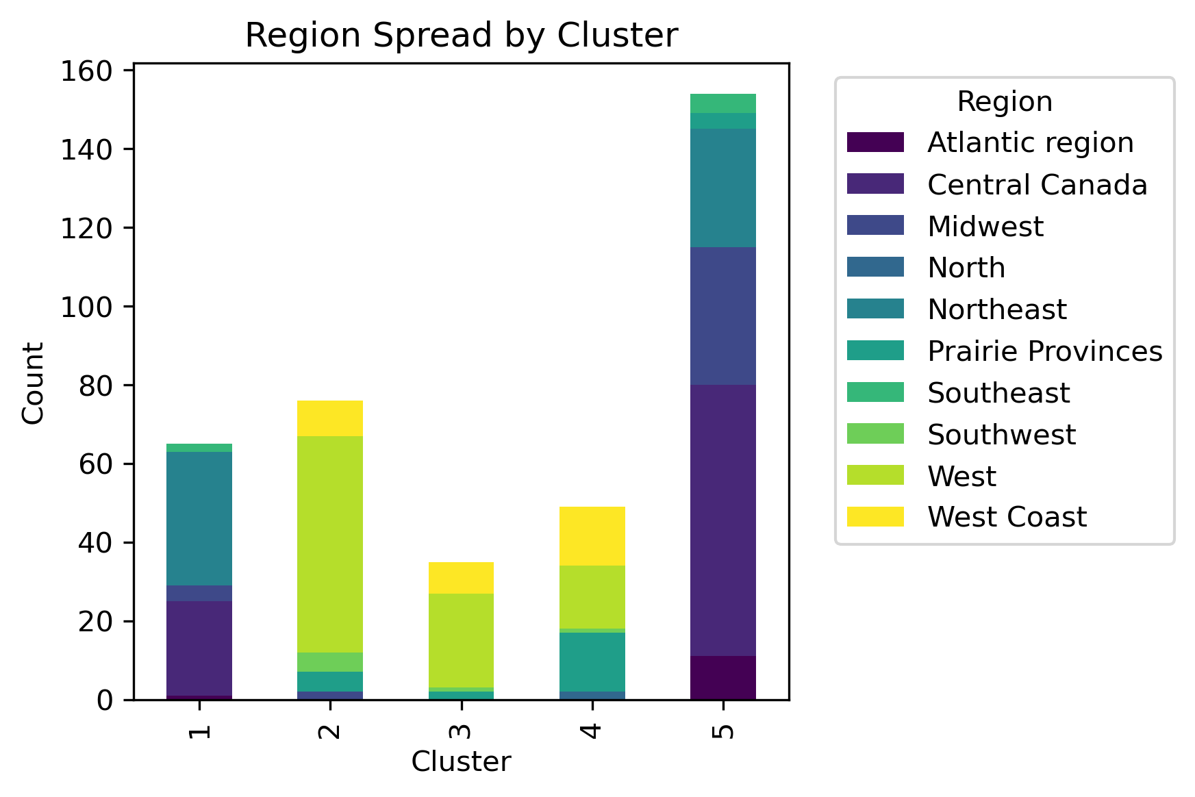
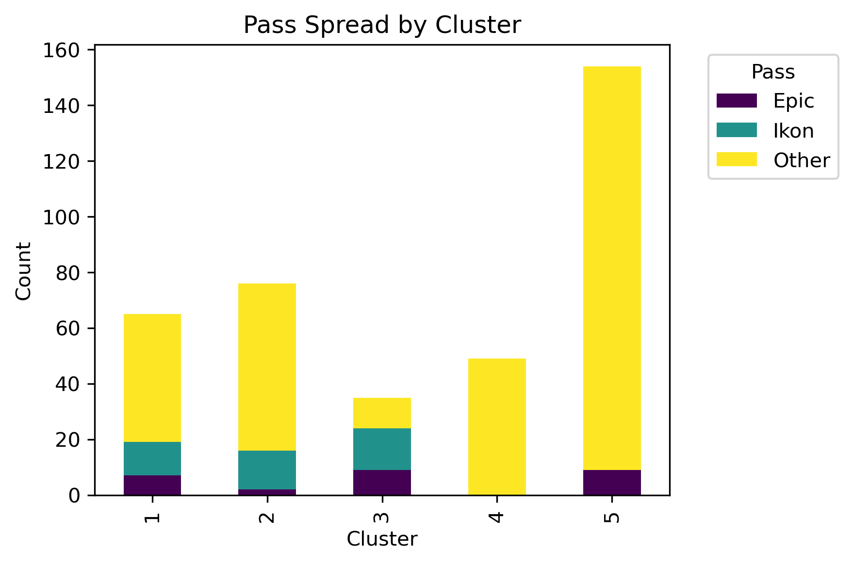
By examining different labels and applying a chi-squared statistic hypothesis test, whether or not a significant association between clusters and column labels can be concluded.
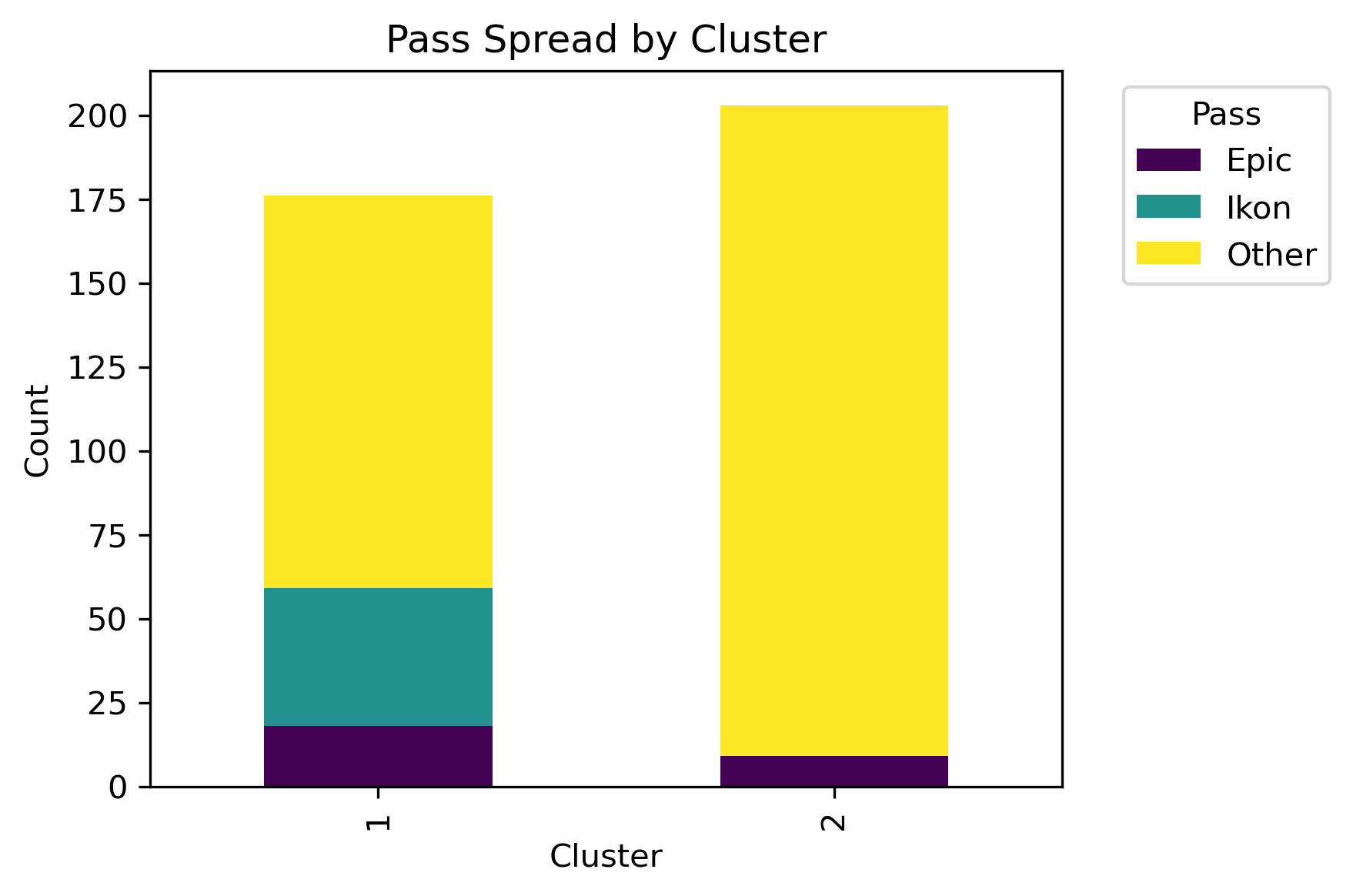
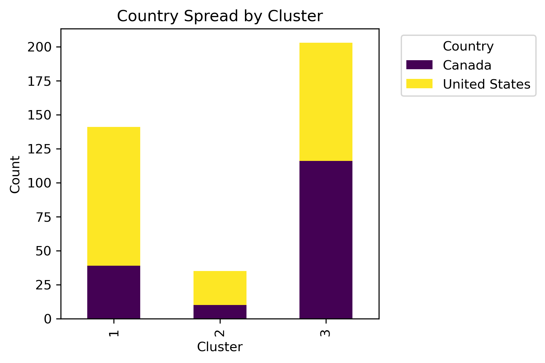
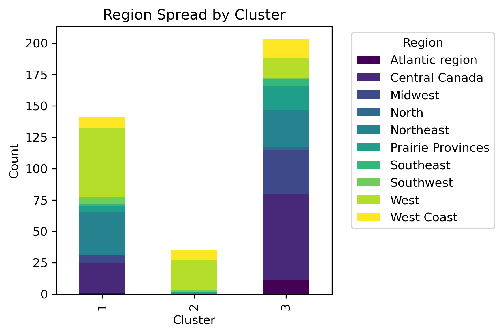
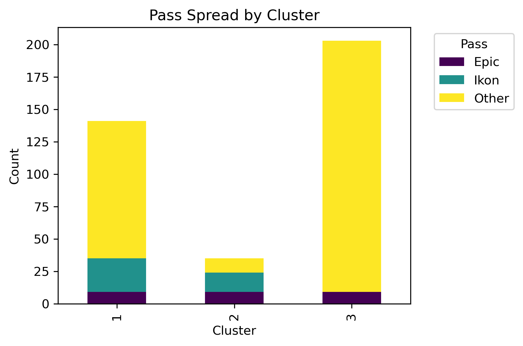
Although there isn't a distinct label separation between the clusters, different distributions of the labels are present in each cluster.
Truncated to Level 3 - Color Threshold set to Distance 30
With a truncation to level 3 revealing a more interpretable dendrogram, further patterns were revealed. By lowering the distance threshold for identifying clusters, different clusters within the data and different distributions can be revealed as well.
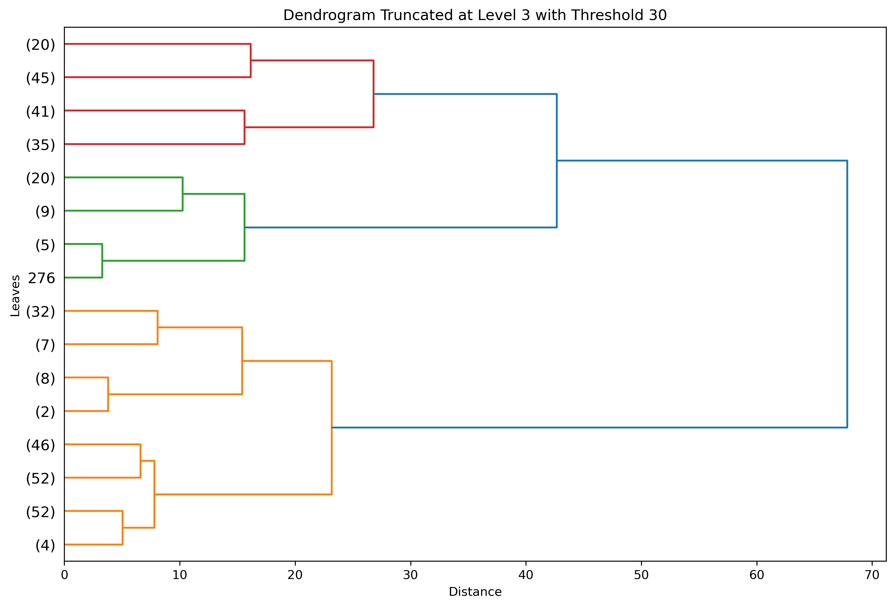
With these parameters, there are three clear clusters. What is underneath the leaves?
Truncated to Level 4 - Color Threshold set to Distance 20
Truncating to Level 3 was vetted well, but further clusters and patterns can be revealed given different parameters. How does a deeper truncation level with a closer distance fair for this data?
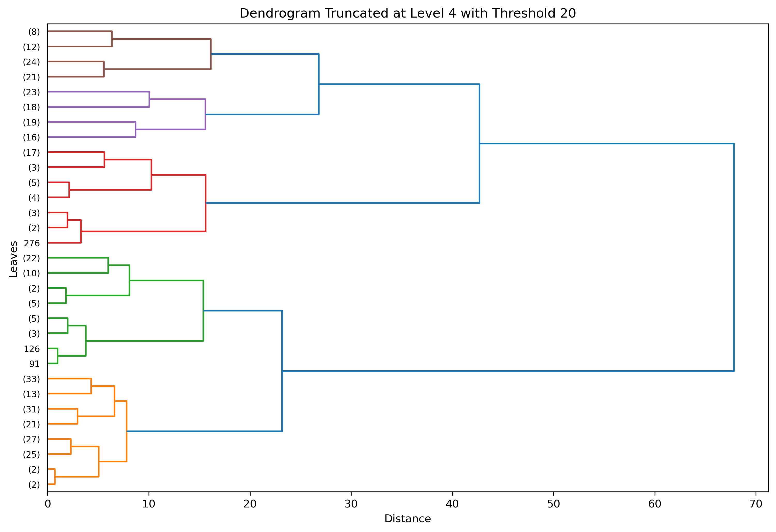
With these parameters, there are five clear clusters. What is underneath the leaves?
Hierarchical Clustering Results and Discussion
Density Clustering (DBSCAN)
Density Clustering is particularly useful when performing clustering on datasets with irregular (arbitrary) shapes and varying densities.
Similar to hierarchical clustering, and different to KMeans clustering, this method doesn't require a specified number of clusters.
The main properties of DBSCAN clustering, comparitively are:
- Arbitrary Cluster Shapes
- Unspecified Number of Clusters
sklearn.cluster.DBSCAN, DBSCAN can be implemented on the datasets associated within this scope. The inputs necessary to utilize this module are namely:
- Epsilon: maximum distance between two observations
- Minimum Samples: number of observations required within parameters to be considered a cluster
Parameter Heuristics
If not utilizing domain knowledge for parameter selection, the following heuristics are generally accepted for density clustering:
- Epsilon: k-distance graph with elbow points
- Minimum Sample: number of dataset dimensions + 1
sklearn.neighbors.NearestNeighbors.
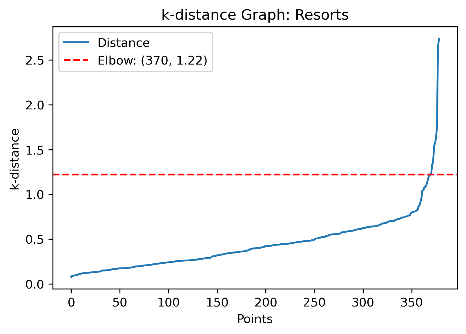
A decent choice for epsilon is then the elbow of the sorted plotted ascending distances.
Finding the elbow, or maximum curvature, can be accomplished through "eyeballing", a manual implementation, or even through a module. This analysis take a manual approach which utilizes KMeans clustering to cluster the slopes between curves and uses an automated approach using
kneed.KneeLocator.
For each dataset, the following parameters will be implemented:
- Manual (i.e. distance slope clustering)
- Automatic (i.e.
KneeLocator) - Custom (i.e. use previous parameters to attempt best clustering)
DBSCAN Clusering - Resorts
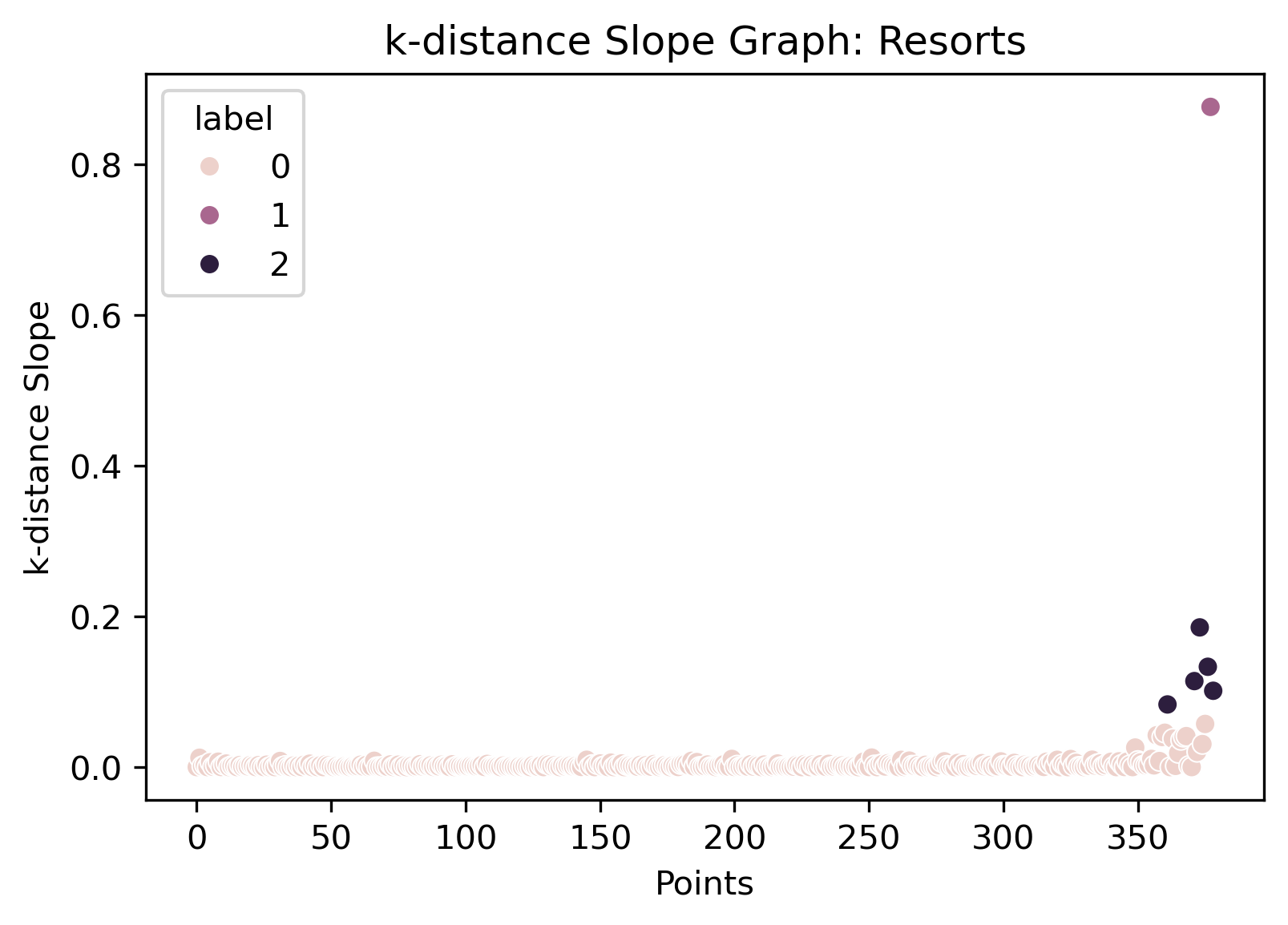
The epsilon value with the automatic detection technique gives a value of 1.22, while looking at the slope clusters give a value of around 0.1. Another manual value for epsilon could be
right where the values start to change on the k-distance graph, which looks to be around 0.8.
By running the DBSCAN algorithm and visually evaluating how the parameters cluster the data can provide insight into the best choice.
DBSCAN Clusering - Weather
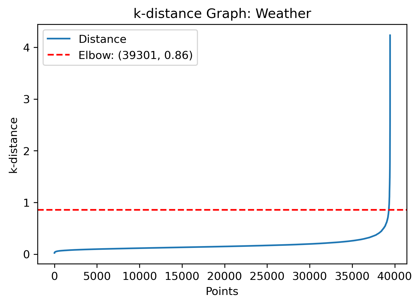
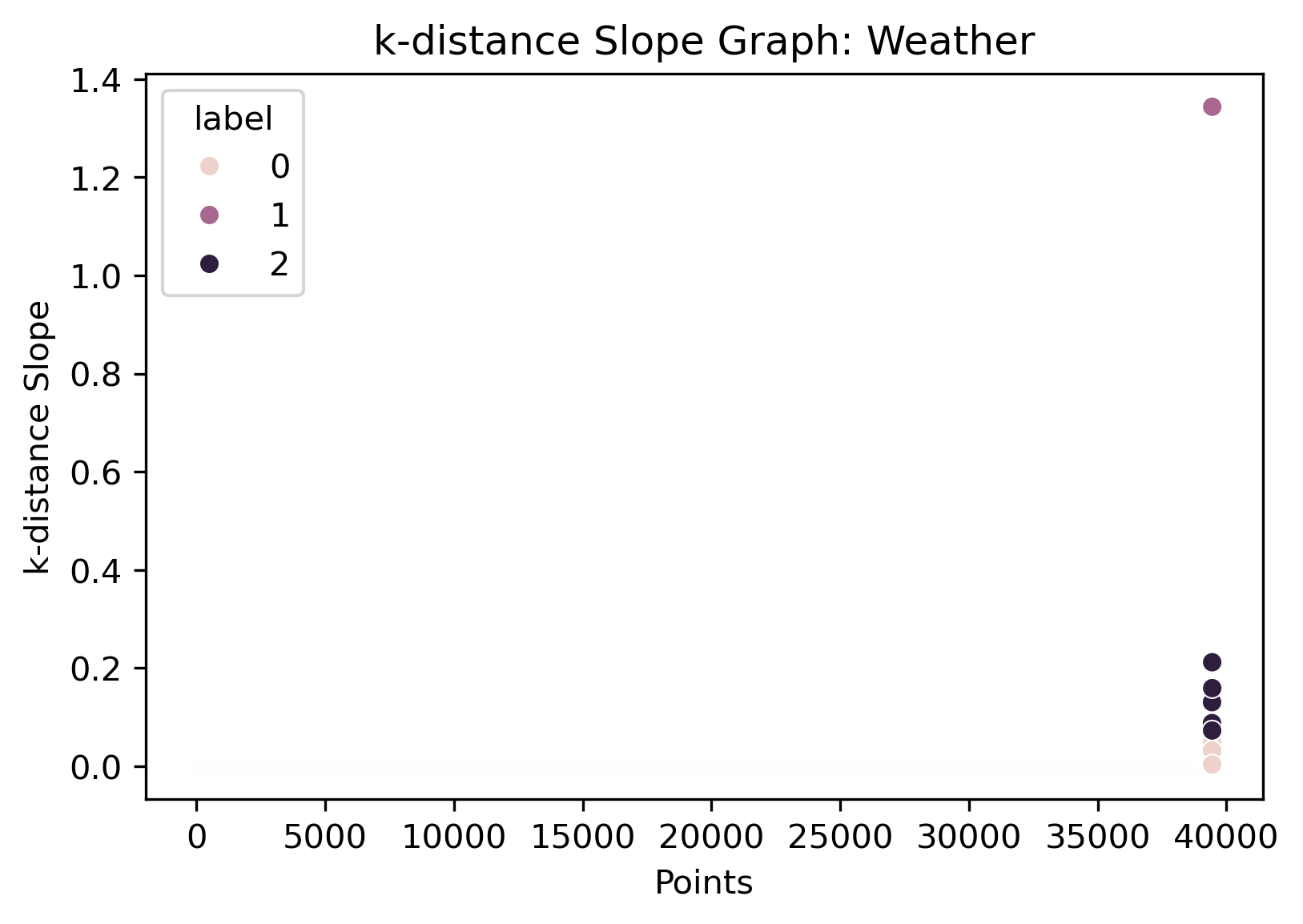
The epsilon value with the automatic detection technique gives a value of 0.86, while looking at the slope clusters give a value of around 0.1. Another manual value for epsilon could be
right where the values start to change on the k-distance graph, which looks to be between these.
By running the DBSCAN algorithm and visually evaluating how the parameters cluster the data can provide insight into the best choice.
DBSCAN Clusering - Google
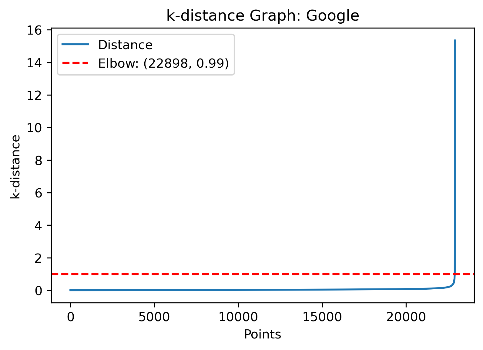
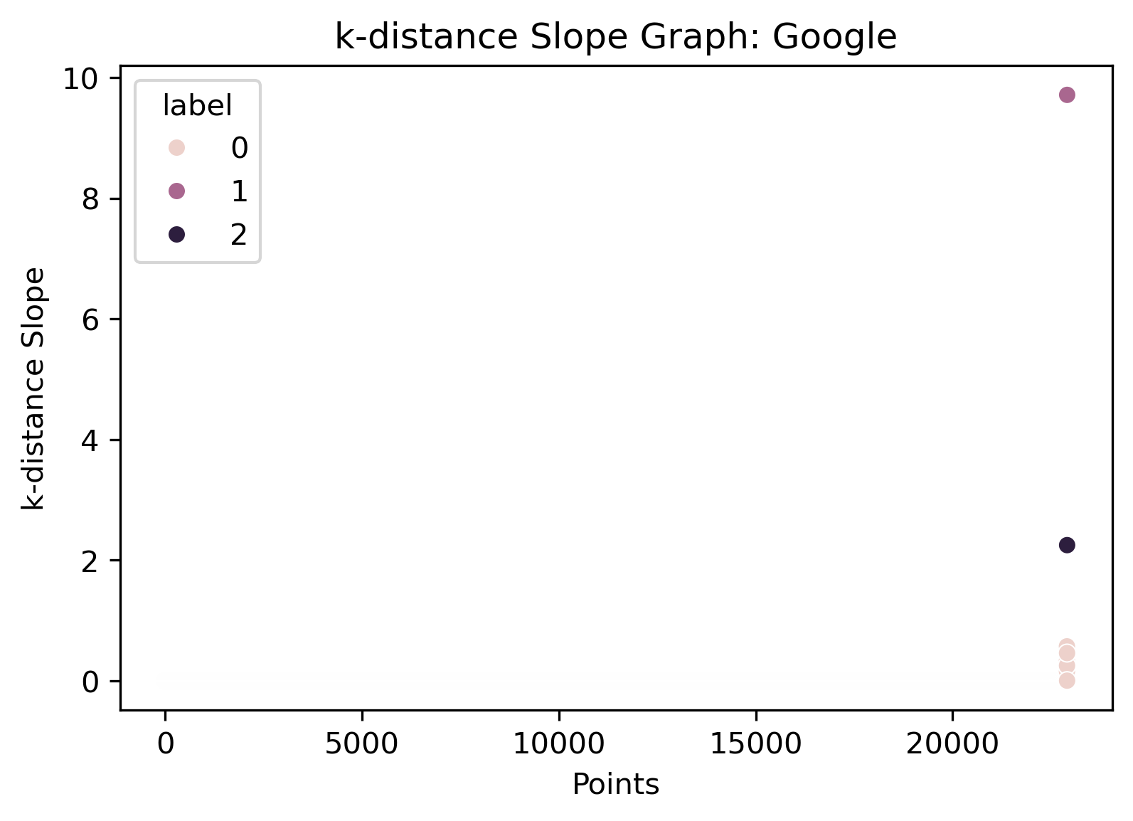
The epsilon value with the automatic detection technique gives a value of 0.99, while looking at the slope clusters give a value of around just above 0 to about 1. A custom version of the parameters was also used
for this with epsilon value of 0.65 and minimum samples of 10.
By running the DBSCAN algorithm and visually evaluating how the parameters cluster the data can provide insight into the best choice.
Density Clustering (DBSCAN) Results and Discussion
Given the arbitrary shape detection used in density clustering, the clustering detection seemed to work best for Resorts Data and
Google Data. A property of this clustering method is its outlier detection. Resorts and Google have rather obscure shapes, especially Google, and it was
mentioned previously that outliers could be causing this. Although these aren't outliers in a typical sense, as they just don't belong any single cluster, its still a decent analysis
technique.
This method wasn't great for the PCA projection of the Weather Data due to its spherical nature. Already being not an obscure shape, the algorithm seemed to cluster itself almost entirely. Although a small change of parameters did result in
some of the datapoints on the outside of the data being grouped together, with more outliers (or not assigned to a single group) were recognized as well.
An Overview on Clustering Techniques (Strengths and Weaknesses)
- KMeans Clustering: iterate through centroids to minimize the sum of square distances between centroids and points.
- Strength: easy to implement and understand.
- Strength: works well with large dataset and relatively quick.
- Weakness: works with the assumption that clusters are spherical and evenly sized.
- Weakness: the number of clusters must be specified beforehand.
- Applications: seemed to work best for the Weather data due its spherical nature.
- Hierarchical Clustering: builds a hierarchy of clusters either bottom-up (agglomerative) or top-down (divisive), which produces a tree structure known as a dendrogram.
- Strength: the dendrogram can produce intuitive visual representations of the data.
- Strength: works with various distance or similarity measures.
- Strength: the shape of the data distribution doesn't affect the results.
- Strength: the number of clusters does not need to be specified beforehand.
- Weakness: computationally expensive.
- Weakness: can be difficult to use on larger datasets.
- Applications: only tested in-depth on the Resort data, which did seem to produce clusters with different properties.
- Density Clustering (DBSCAN): groups together closely packed points and identifies areas of high density as clusters based on parameters.
- Strength: the number of clusters does not need to be specified beforehand.
- Strength: works well with clusters of arbitrary shape.
- Weakness: the process is highly sensitive to parameter choice, which are given in place of a specified number of clusters.
- Weakness: computationally expensive
- Applications: seemed to work best for the Resort and Google data, which is logical due to their arbitrary and obsure shapes. This did not work well on the Weather data, likely due to the entirety of the data essentially being a highly dense sphere.
Conclusion
Distinct groupings can be identified for staple sources associated with the ski and snowbound community. Ski Resorts themselves, Weather Phenomena surrounding Ski Resorts, and Places of Business all contain characteristics which can be consolidated and patterns extracted. Ski Resorts can be processed into hierarchical structure which explains different distributions such as location (either county or region) or by Pass Type (Ikon, Epic, Other). Weather characteristics tend to form patterns around the type of weather (snow, rain, clear, etc.) and especially around time of year (i.e. months). Places of Business tend to form different groups based on their category, location (either county or region), and even by the Pass Type (Ikon, Epic, Other) of their associated ski resort!
