Modeling - PRincipal Component Analysis (PCA)
What is PCA?
Principal Component Analysis, or simply PCA, is a dimenson reduction technique which operates by consolidating information from multiple features into a new projection space in which each new feature is orthogonal to each other new feature. Specifically, PCA is a constrained optimization technique in which an eigenspace transformation is used to put quantitative data into a different orthonormal basis. PCA initialization requires standardization (which limits the variation of the data), from which a covariance matrix is computed. The eigenspace transformation extracts eigenvalues and eigenvectors from the covariance matrix of the standardized data. The covariance matrix step is crucial, as antyhing above a zero shows correlation, which is what needs to removed. In essence, the eigenvectors form the orthonormal basis due to them being uncorrelated. The associated eigenvalues are the explained information (or explained variance) of the eigenvectors. In a dataset which has no correlation between its variables, the eigenvectors would essentially be its columns and removing dimensions removes actual information. However, this is rare in real datasets. Furthermore, the covariance matrix is symmetric, which allows for the guaranteed existence of an orthonormal basis of corresponding vector space consisting of eigenvectors and corresponding real-valued eigenvalues.
What Data Can Be Used?
PCA is used on quantitative data. This analysis focuses on the quantitative data of the main datasets used throughout this project:
Ski Resorts Data - Snippet
| Resort | state_province_territory | Country | City | Overall Rating | Elevation Difference | Elevation Low | Elevation High | Trails Total | Trails Easy | Trails Intermediate | Trails Difficult | Lifts | Price | Resort Size | Run Variety | Lifts Quality | Latitude | Longitude | Pass | Region |
|---|---|---|---|---|---|---|---|---|---|---|---|---|---|---|---|---|---|---|---|---|
| 49 Degrees North Mountain Resort | Washington | United States | Chewelah | 3.4 | 564 | 1196 | 1760 | 68.0 | 20.0 | 27.0 | 21.0 | 7 | 82.0 | 3.5 | 4.0 | 3.3 | 48.277375 | -117.701815 | Other | West |
| Crystal Mountain (WA) | Washington | United States | Sunrise | 3.3 | 796 | 1341 | 2137 | 50.0 | 8.0 | 27.0 | 15.0 | 11 | 199.0 | 3.2 | 3.6 | 3.7 | 46.928167 | -121.504535 | Ikon | West |
| Mt. Baker | Washington | United States | White Salmon | 3.4 | 455 | 1070 | 1525 | 100.0 | 24.0 | 45.0 | 31.0 | 10 | 91.0 | 3.9 | 4.3 | 3.0 | 45.727775 | -121.486699 | Other | West |
| Mt. Spokane | Washington | United States | Mead | 3.0 | 610 | 1185 | 1795 | 26.0 | 6.5 | 16.0 | 3.5 | 7 | 75.0 | 2.7 | 3.1 | 3.0 | 47.919072 | -117.092505 | Other | West |
| Sitzmark | Washington | United States | Tonasket | 2.6 | 155 | 1330 | 1485 | 7.5 | 2.0 | 3.0 | 2.5 | 2 | 50.0 | 1.9 | 2.4 | 2.9 | 48.863907 | -119.165077 | Other | West |
| Stevens Pass | Washington | United States | Baring | 3.3 | 580 | 1170 | 1750 | 39.0 | 6.0 | 18.0 | 15.0 | 10 | 119.0 | 3.1 | 3.5 | 3.6 | 47.764031 | -121.474822 | Epic | West |
| The Summit at Snoqualmie | Washington | United States | Snoqualmie Pass | 3.0 | 380 | 800 | 1180 | 27.9 | 5.2 | 13.7 | 9.0 | 22 | 135.0 | 2.6 | 3.0 | 3.2 | 47.405235 | -121.412783 | Ikon | West |
| Wenatchee Mission Ridge | Washington | United States | Wenatchee | 3.2 | 686 | 1392 | 2078 | 36.0 | 4.0 | 21.0 | 11.0 | 4 | 119.0 | 2.9 | 3.3 | 3.6 | 47.292466 | -120.399871 | Other | West |
| Abenaki | New Hampshire | United States | Wolfeboro | 2.1 | 70 | 180 | 250 | 2.0 | 1.2 | 0.5 | 0.3 | 1 | 24.0 | 1.4 | 1.8 | 1.4 | 43.609528 | -71.229692 | Other | Northeast |
| Attitash Mountain Resort | New Hampshire | United States | Bartlett | 3.2 | 533 | 183 | 716 | 37.0 | 7.4 | 17.4 | 12.2 | 8 | 129.0 | 2.9 | 3.3 | 3.7 | 44.084603 | -71.221525 | Epic | Northeast |
Weather Data - Snippet
| datetime | tempmax | tempmin | temp | feelslikemax | feelslikemin | feelslike | dew | humidity | precip | precipprob | precipcover | snow | snowdepth | windgust | windspeed | winddir | pressure | cloudcover | visibility | solarradiation | solarenergy | uvindex | sunrise | sunset | moonphase | icon | stations | resort | tzoffset | severerisk | type_freezingrain | type_ice | type_none | type_rain | type_snow |
|---|---|---|---|---|---|---|---|---|---|---|---|---|---|---|---|---|---|---|---|---|---|---|---|---|---|---|---|---|---|---|---|---|---|---|---|
| 2019-01-01 | 16.4 | 2.0 | 7.0 | 10.2 | -13.3 | -0.6 | -1.2 | 69.1 | 0.008 | 100.0 | 20.83 | 0.0 | 20.7 | 18.30000 | 10.6 | 4.9 | 1014.5 | 59.0 | 8.6 | 116.8 | 9.9 | 5.0 | 07:26:20 | 16:51:51 | 0.85 | snow | ['72467523063', '72206103038', 'CACMC', 'KCCU', 'KEGE', 'KLXV', 'DJTC2', 'K20V', '72467393009'] | Vail | 0.0 | 0.0 | 0 | 0 | 0 | 0 | 1 |
| 2019-01-02 | 24.3 | -0.9 | 11.4 | 21.9 | -11.9 | 5.4 | -10.5 | 39.9 | 0.004 | 100.0 | 4.17 | 0.0 | 20.8 | 29.77377 | 8.7 | 353.1 | 1021.4 | 0.0 | 9.9 | 121.6 | 10.7 | 5.0 | 07:26:27 | 16:52:41 | 0.89 | snow | ['72467523063', '72206103038', 'CACMC', 'KCCU', 'KEGE', 'KLXV', 'DJTC2', 'K20V', '72467393009'] | Vail | 0.0 | 0.0 | 0 | 0 | 0 | 0 | 1 |
| 2019-01-03 | 29.0 | 5.3 | 17.6 | 21.9 | -4.0 | 8.6 | 4.1 | 56.1 | 0.004 | 100.0 | 4.17 | 0.2 | 20.8 | 32.20000 | 9.8 | 328.9 | 1024.7 | 0.0 | 9.8 | 123.3 | 10.6 | 5.0 | 07:26:31 | 16:53:33 | 0.92 | snow | ['72467523063', '72206103038', 'CACMC', 'KCCU', 'KEGE', 'KLXV', 'DJTC2', 'K20V', '72467393009'] | Vail | 0.0 | 0.0 | 0 | 0 | 0 | 1 | 1 |
| 2019-01-04 | 34.0 | 11.9 | 23.4 | 28.7 | 3.4 | 17.1 | 7.0 | 50.4 | 0.001 | 100.0 | 4.17 | 0.1 | 20.8 | 20.80000 | 9.0 | 311.0 | 1025.5 | 0.0 | 9.9 | 123.7 | 10.7 | 5.0 | 07:26:34 | 16:54:26 | 0.96 | snow | ['72467523063', '72206103038', 'CACMC', 'KCCU', 'KEGE', 'KLXV', 'DJTC2', 'K20V', '72467393009'] | Vail | 0.0 | 0.0 | 0 | 0 | 0 | 1 | 1 |
| 2019-01-05 | 34.1 | 14.3 | 27.1 | 29.4 | 4.3 | 20.1 | 1.9 | 33.9 | 0.001 | 100.0 | 4.17 | 0.0 | 20.4 | 20.80000 | 10.1 | 243.5 | 1022.2 | 19.4 | 9.7 | 110.3 | 9.6 | 5.0 | 07:26:34 | 16:55:20 | 0.00 | rain | ['72467523063', '72206103038', 'CACMC', 'DYGC2', 'KCCU', 'KEGE', 'KLXV', 'DJTC2', 'K20V', '72467393009'] | Vail | 0.0 | 0.0 | 0 | 0 | 0 | 1 | 1 |
| 2019-01-06 | 29.9 | 18.5 | 25.9 | 22.4 | 5.1 | 16.1 | 18.1 | 72.5 | 0.035 | 100.0 | 58.33 | 0.6 | 20.6 | 33.30000 | 16.9 | 266.7 | 1009.3 | 78.7 | 6.3 | 47.3 | 4.1 | 2.0 | 07:26:32 | 16:56:16 | 0.02 | snow | ['72467523063', '72206103038', 'CACMC', '72038500419', 'DYGC2', 'KCCU', 'KEGE', 'A0000594076', 'KLXV', 'DJTC2', 'K20V', '72467393009'] | Vail | 0.0 | 0.0 | 0 | 0 | 0 | 1 | 1 |
| 2019-01-07 | 24.8 | 14.7 | 20.3 | 12.8 | 2.5 | 6.5 | 13.7 | 75.2 | 0.004 | 100.0 | 8.33 | 0.4 | 21.3 | 45.70000 | 27.9 | 271.2 | 1015.6 | 83.7 | 4.8 | 35.8 | 3.0 | 2.0 | 07:26:27 | 16:57:13 | 0.06 | snow | ['72467523063', '72206103038', 'CACMC', 'DYGC2', 'KCCU', 'KEGE', 'KLXV', 'DJTC2', 'K20V', '72467393009'] | Vail | 0.0 | 0.0 | 0 | 0 | 0 | 0 | 1 |
| 2019-01-08 | 34.6 | 17.2 | 25.1 | 34.6 | 5.0 | 17.8 | 12.0 | 59.5 | 0.013 | 100.0 | 8.33 | 0.0 | 21.3 | 27.70000 | 15.2 | 312.1 | 1029.4 | 34.5 | 9.5 | 122.9 | 10.5 | 5.0 | 07:26:21 | 16:58:11 | 0.09 | rain | ['72467523063', '72206103038', 'CACMC', 'KCCU', 'KEGE', 'KLXV', 'DJTC2', 'K20V', '72467393009'] | Vail | 0.0 | 0.0 | 0 | 0 | 0 | 1 | 1 |
| 2019-01-09 | 38.3 | 23.0 | 28.6 | 38.3 | 13.6 | 22.6 | 9.9 | 45.4 | 0.000 | 0.0 | 0.00 | 0.0 | 21.2 | 23.00000 | 13.0 | 142.9 | 1029.6 | 1.0 | 9.9 | 114.0 | 9.8 | 5.0 | 07:26:12 | 16:59:11 | 0.12 | clear-day | ['72467523063', '72206103038', 'CACMC', 'KCCU', 'KEGE', 'KLXV', 'DJTC2', 'K20V', '72467393009'] | Vail | 0.0 | 0.0 | 0 | 0 | 1 | 0 | 0 |
| 2019-01-10 | 33.7 | 17.0 | 26.4 | 33.7 | 9.8 | 22.6 | 14.3 | 60.6 | 0.026 | 100.0 | 12.50 | 0.8 | 21.4 | 17.20000 | 8.8 | 323.7 | 1023.3 | 39.9 | 8.3 | 75.9 | 6.6 | 4.0 | 07:26:01 | 17:00:11 | 0.16 | snow | ['72467523063', '72206103038', 'CACMC', 'KCCU', 'KEGE', 'KLXV', 'DJTC2', 'K20V', '72467393009'] | Vail | 0.0 | 0.0 | 0 | 0 | 0 | 1 | 1 |
Google Places Data - Snippet
| Latitude | Longitude | Name | rating | total_ratings | Resort | Call Category | Initial Category | Secondary Category | Tertiary Category |
|---|---|---|---|---|---|---|---|---|---|
| 39.639411 | -106.367836 | Manor Vail Lodge | 4.7 | 370.0 | Vail | Restaurants | bar | lodging | restaurant |
| 39.641578 | -106.371678 | Gravity Haus Vail | 4.4 | 256.0 | Vail | Restaurants | gym | spa | lodging |
| 39.642639 | -106.377803 | Leonora | 4.3 | 167.0 | Vail | Restaurants | restaurant | food | point_of_interest |
| 39.638962 | -106.369379 | Larkspur Events & Dining | 4.5 | 198.0 | Vail | Restaurants | restaurant | food | point_of_interest |
| 39.630370 | -106.418694 | Subway | 2.7 | 105.0 | Vail | Restaurants | meal_takeaway | restaurant | food |
| 39.640861 | -106.374665 | Sweet Basil | 4.4 | 838.0 | Vail | Restaurants | bar | restaurant | food |
| 39.640228 | -106.374381 | Elway's | 4.3 | 385.0 | Vail | Restaurants | bar | restaurant | food |
| 39.643914 | -106.390088 | The Little Diner | 4.7 | 1390.0 | Vail | Restaurants | restaurant | food | point_of_interest |
| 39.640248 | -106.373333 | Red Lion | 3.9 | 740.0 | Vail | Restaurants | bar | restaurant | food |
| 39.641490 | -106.397471 | Chicago Pizza | 3.9 | 216.0 | Vail | Restaurants | meal_delivery | meal_takeaway | restaurant |
Data Preparation
Each dataset required some alteration in preparation for PCA. Namely, this included subsetting the data to quantitative values and separating the labels. The labels would be saved for later to compare with the results. Some of the datasets had multiple categorical data features which could be used as labels depending on the purpose of the analysis. Other columns were simply dropped. Thus, a concise script with which could perform this cleaning, along with applying the PCA algorithm and analysis of the results was created. This script can be found here, and contains detailed documentation on these functions.
Ski Resort Data - Preparation
- Quantitative Data Retained:
- Overall Rating
- Elevation Difference
- Elevation Low
- Elevation High
- Trails Total
- Trails Easy
- Trails Intermediate
- Trails Difficult
- Lifts
- Price
- Resort Size
- Run Variety
- Lifts Quality
- Latitude
- Longitude
- Potential Label Columns Set Aside:
- Resort
- state_province_territory
- Country
- City
- Pass
- Region
Weather Data - Preparation
- Quantitative Data Retained:
- tempmax
- tempmin
- temp
- feelslikemax
- feelslikemin
- feelslike
- dew
- humidity
- precip
- snow
- snowdepth
- windgust
- windspeed
- winddir
- pressure
- cloudcover
- visibility
- solarradiation
- solarenergy
- uvindex
- moonphase
- severerisk
- Potential Label Columns Set Aside:
- datetime
- icon
- resort
- type_snow
- type_rain
- type_ice
- type_freezingrain
- type_none
Google Places Data - Preparation
- Quantitative Data Retained:
- Latitude
- Longitude
- rating
- total_ratings
- Potential Label Columns Set Aside:
- Name
- Resort
- Call Category
- Initial Category
- Secondary Category
- Tertiary Category
Applying Principal Component Analysis in Python
PCA in Python can be accomplished through the Scikit-Learn module, sklearn.decomposition.PCA. However, it is important
to first normalize the quantitative data. Results can be skewed when values are significantly different between features. In other words,
when features have much larger and smaller values than each other. To accomplish normalization, another Scikit-Learn module was used,
sklearn.preprocessing.StandardScaler. Each feature has its mean removed and is scaled to unit variance.
PCA can be applied in a generic sense, without specifying how many principal components are to be returned. This will create a return of
as many principal components as there are input features. PCA can also be applied with a desired number of components to be returned. One point of confusion with
either of these methods is how the original features relate to the output. It's important to understand that PCA transforms or projects the data into a different space using
eigenvalues and eigenvectors. There isn't exactly a one-to-one relationship between the projected data onto principal components and the features of the original dataset. To
further illustrate PCA, analyze its results, and try to make sense of a relationship between original features and the PCA projection, several attributes of sklearn's PCA model
will be used. Given a model was created with the following code:
        # sklearn libraries
        from sklearn.decomposition import PCA
        from sklearn.preprocessing import StandardScaler

        # normalize pandas dataframe with only quantitative features
        scaler = StandardScaler()
        df_normal = scaler.fit_transform(df)

        # create the pca model and project data into PCA space
        pca = PCA()
        pca_projection = pca.fit_transform(df_normal)

        # obtain eigenvalues
        eigenvalues = pca.explained_variance_

        # explained variance
        eigenvalue_ratios = pca.explained_variance_ratio_

        # obtain eigenvectors
        eigenvectors = pca.components_

        # obtain loadings matrix
        loadings_matrix = pd.DataFrame(pca.components_.T, columns=[f'principal_component_{col+1}' for col in range(pca.components_.shape[0])], index=df.columns)
Attributes Explained:
- eigenvalues: the amount of variance explained by each of the selected components
- eigenvectors: directions of maximum variance in the data, sorted by decreasing eigenvalues
- eigenvalue ratios: percentage of variance explained by each of the selected components
- loadings matrix: represents the correlation between original features and principal components
- pca projection: original data projected onto the pca space
PCA and Analysis Process
Each dataset was processed and the results were analyzed in this script,
for full-feature PCA, 3-dimensional PCA, and 2-dimensional PCA via the following:
- PCA Application and Key Attribute Extraction
perform_pca() - Orthogonality Validated
validate_orthogonality() - Visualize Variance
visualize_variance() - Full Dimensional PCA Includes Additional Outputs for Components Required for Retention of 95% Explained Variance
- Explained Variance
- Full Dimensional PCA Includes Additional Output for the Top 3 Eigenvalues
- Loadings Matrix Analysis
- Loadings Matrix Barplot
- Loadings Matrix Boxplot
- Further Visualizations
- 3-Dimensional PCA with Labeled Hue - Weather Includes an Animated Time Series Visualization
- 2-Dimensional PCA with Labeled Hue
The Loadings Matrix
Loadings Matrices represent the correlation between the original variables and the principal components. When PCA is performed,
the new principal components are a consolidation of information of the original variables. Therefore, each principal component could be influenced by each of the original variables (i.e. potentially contain information from each original variable).
The loadings matrix shows this influence (direction and strength) amount by calculating correlations. Closer to zero, the less influence. A positive correlation indicates that higher scores on the factor are associated with higher scores on the variable.
A negative correlation indicates that higher scores on the factor are associated with lower scores on the variable. Higher negative correlations (in an absolute sense) are indicative of high influence, just inversely!
Essentially, these correlations help in understanding which factors influence which variables and whether this influence is direct or inverse. By analyzing loadings matrices, the true power of PCA and its consolidation properties are revealed.
To further illustrate this property, it can be beneficial to investigate the absolute values of a loadings matrix. Using absolute values, the correlations will be investigated via the following:
- Correlation Ranking
- Turn correlations into their absolute value correlations.
- Obtain rank of each original variable across each principal component. The lower the rank, the higher the absolute correlation, the more influenced a principal component is by the original variable.
- Analyze the rankings
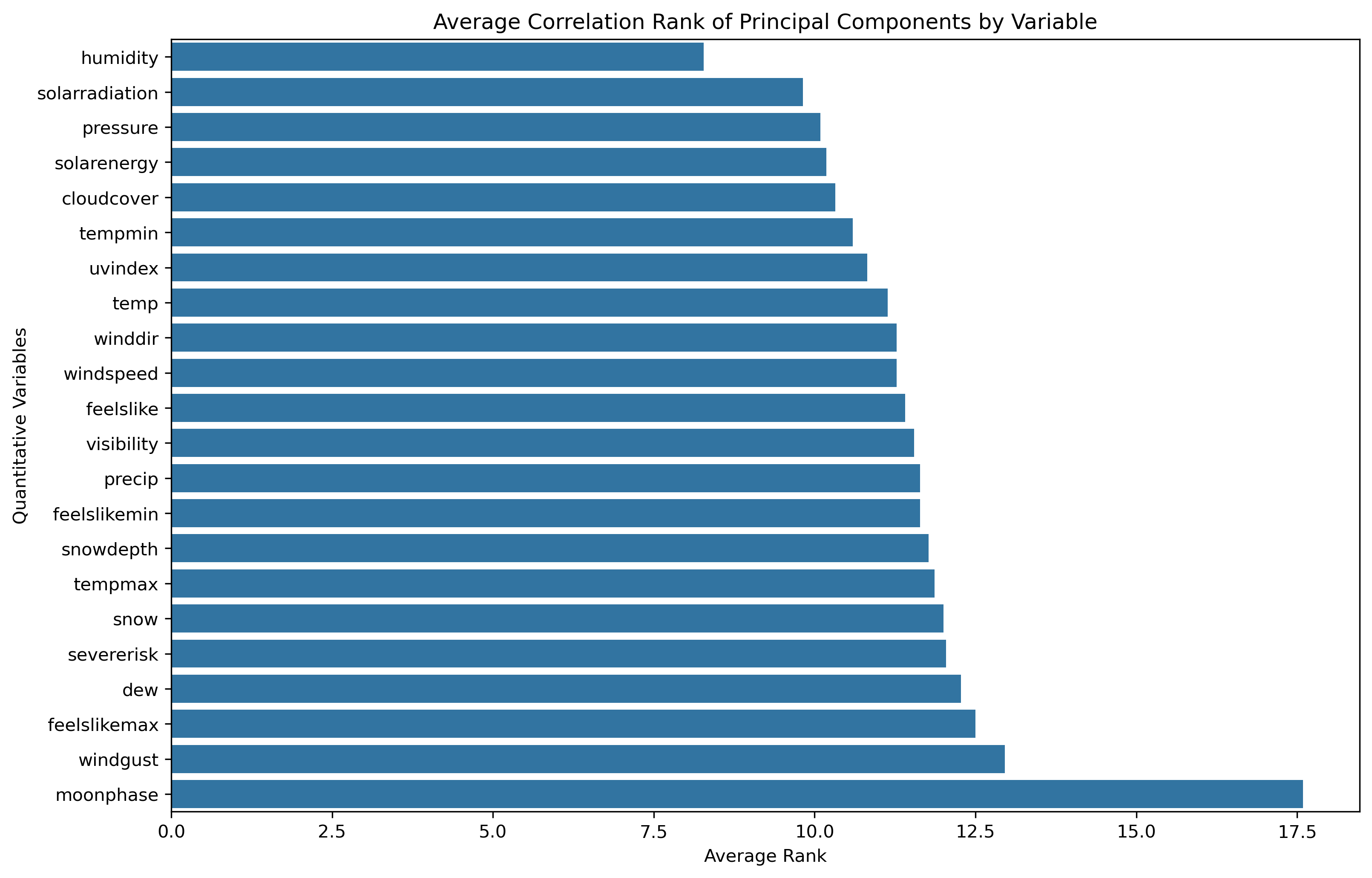
- Average Correlation Ranking: a low average absolute correlation rank indicates this original variable has greater influence across the principal components, thus a more substantial amount of information is obtained from that original variable.
- Correlation Ranking Spread: a mean is a common statistical measure, but the overall spread of rankings can illustrate further statistical measures and influence as a whole.
PCA Results and Analysis
Explained and Cumulative Variance - Table
| principal_components | explained_variance | cumulative_variance |
|---|---|---|
| principal_component_1 | 67.37% | 67.37% |
| principal_component_2 | 9.88% | 77.25% |
| principal_component_3 | 8.37% | 85.63% |
| principal_component_4 | 4.34% | 89.97% |
| principal_component_5 | 2.80% | 92.77% |
| principal_component_6 | 2.11% | 94.88% |
| principal_component_7 | 1.38% | 96.26% |
| principal_component_8 | 0.97% | 97.23% |
| principal_component_9 | 0.86% | 98.09% |
| principal_component_10 | 0.77% | 98.85% |
| principal_component_11 | 0.67% | 99.52% |
| principal_component_12 | 0.34% | 99.86% |
| principal_component_13 | 0.14% | 100.00% |
| principal_component_14 | 0.00% | 100.00% |
| principal_component_15 | 0.00% | 100.00% |
Explained and Cumulative Variance - Visual
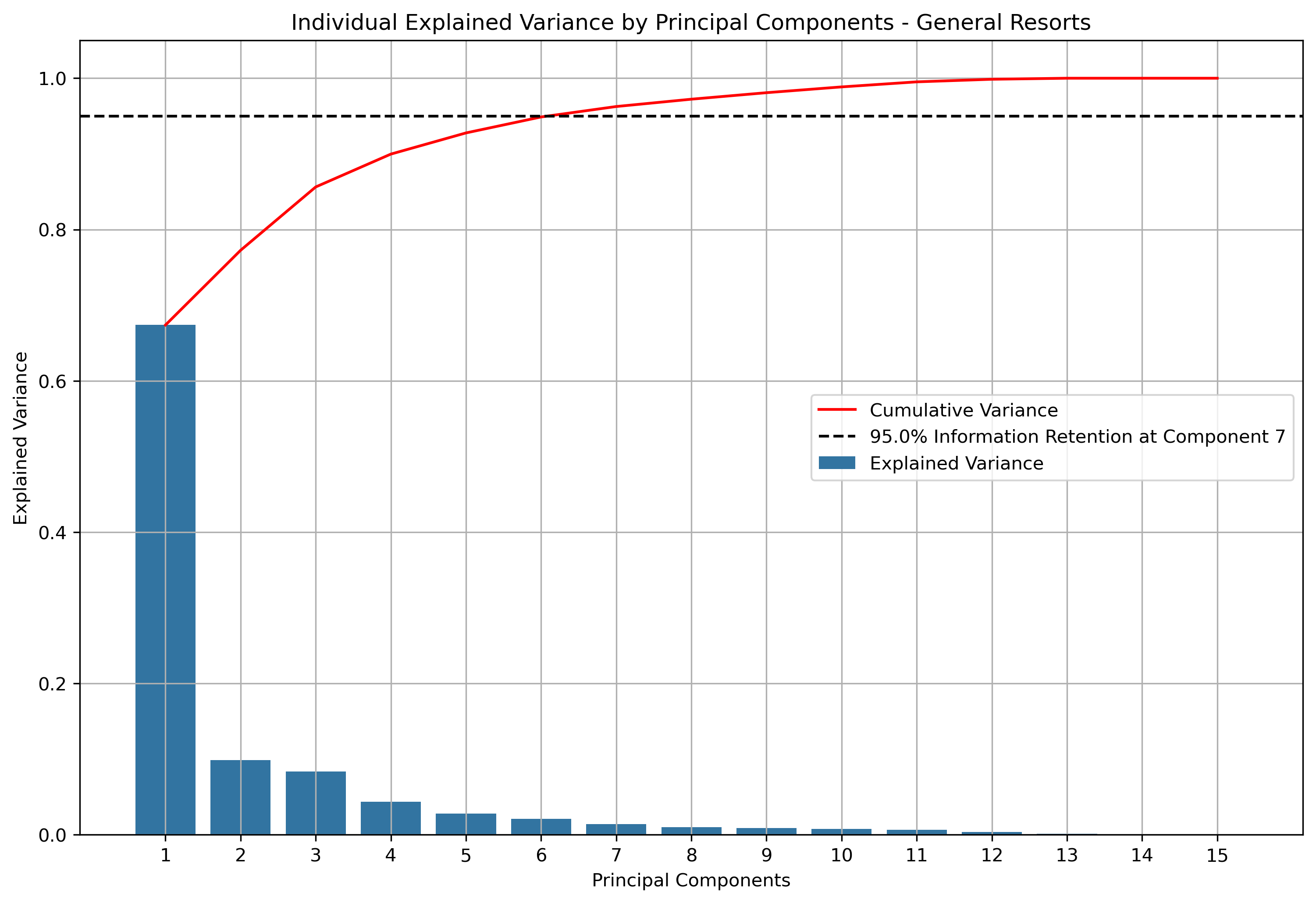
Illustrated above is how much information is retained or explained by each principal component. The principal components are ordered by descending associated eigenvalues, such that the principal component with the largest associated eigenvalue is first. This means that the principal components decreasingly explain the variance in the dataset. For this particular dataset, it takes 7 principal components until 95% of variance within the dataset is explained.
Eigenvalues - Python Output
print(pca.explained_variance_)
Eigenvalues Results:
[1.01328995e+01
 1.48572492e+00
 1.25942178e+00
 6.53151568e-01
 4.20975982e-01
 3.17249298e-01
 2.07698104e-01
 1.45693923e-01
 1.29290376e-01
 1.15058542e-01
 1.00412733e-01
 5.16338499e-02
 2.04720021e-02
 1.69084120e-16
 0.00000000e+00]
Eigenvalues - Table
| Principal Component | Eigenvalue |
|---|---|
| Principal Component 1 | 1.013290e+01 |
| Principal Component 2 | 1.485725e+00 |
| Principal Component 3 | 1.259422e+00 |
| Principal Component 4 | 6.531516e-01 |
| Principal Component 5 | 4.209760e-01 |
| Principal Component 6 | 3.172493e-01 |
| Principal Component 7 | 2.076981e-01 |
| Principal Component 8 | 1.456939e-01 |
| Principal Component 9 | 1.292904e-01 |
| Principal Component 10 | 1.150585e-01 |
| Principal Component 11 | 1.004127e-01 |
| Principal Component 12 | 5.163385e-02 |
| Principal Component 13 | 2.047200e-02 |
| Principal Component 14 | 1.690841e-16 |
| Principal Component 15 | 0.000000e+00 |
The highest 3 eigenvalues for this dataset are:
- 10.1328995
- 1.48572492
- 1.25942178
Loadings - Table
| Feature | principal_component_1 | principal_component_2 | principal_component_3 | principal_component_4 | principal_component_5 | principal_component_6 | principal_component_7 | principal_component_8 | principal_component_9 | principal_component_10 | principal_component_11 | principal_component_12 | principal_component_13 | principal_component_14 | principal_component_15 |
|---|---|---|---|---|---|---|---|---|---|---|---|---|---|---|---|
| Overall Rating | 0.295563 | 0.128409 | 0.070401 | 0.232184 | -0.094052 | -0.041479 | -0.099155 | 0.072975 | -0.378219 | 0.150935 | 0.063638 | -0.559794 | -0.572987 | 7.456905e-15 | 7.670563e-15 |
| Elevation Difference | 0.286191 | 0.006434 | 0.127605 | 0.167531 | -0.228009 | -0.190198 | -0.369776 | -0.253744 | 0.513513 | -0.391630 | -0.319654 | -0.107830 | -0.056779 | 5.110595e-03 | -2.242655e-01 |
| Elevation Low | 0.217565 | -0.531208 | -0.238126 | -0.001341 | -0.089008 | -0.004357 | 0.195668 | -0.019658 | -0.169175 | -0.211791 | 0.346592 | 0.038955 | -0.001744 | 1.389608e-02 | -6.097944e-01 |
| Elevation High | 0.259075 | -0.424419 | -0.153443 | 0.048371 | -0.138730 | -0.059634 | 0.047891 | -0.090669 | 0.015794 | -0.285562 | 0.183808 | -0.000564 | -0.018158 | -1.731504e-02 | 7.598268e-01 |
| Trails Total | 0.300028 | 0.106896 | 0.083704 | -0.253912 | -0.012046 | -0.099508 | 0.264873 | 0.083491 | 0.147917 | 0.083732 | 0.012235 | -0.051628 | 0.036309 | 8.405429e-01 | 1.915441e-02 |
| Trails Easy | 0.262651 | 0.127329 | 0.075640 | -0.169168 | -0.242956 | 0.807016 | 0.248873 | -0.152756 | 0.202290 | 0.040188 | 0.013476 | -0.089427 | -0.010379 | -1.845217e-01 | -4.204907e-03 |
| Trails Intermediate | 0.289896 | 0.097366 | 0.072066 | -0.186081 | 0.097909 | -0.193740 | 0.056222 | 0.699348 | 0.326742 | -0.028557 | 0.207625 | -0.161966 | 0.140197 | -3.614567e-01 | -8.236928e-03 |
| Trails Difficult | 0.276246 | 0.087010 | 0.084746 | -0.320954 | -0.001912 | -0.453792 | 0.436673 | -0.431162 | -0.086834 | 0.204626 | -0.187773 | 0.088369 | -0.050931 | -3.581472e-01 | -8.161508e-03 |
| Lifts | 0.251273 | 0.201499 | -0.109092 | -0.344663 | 0.601134 | 0.153135 | -0.239592 | -0.114220 | -0.301317 | -0.459604 | -0.063076 | -0.041792 | 0.050510 | 2.745585e-16 | 6.575543e-16 |
| Price | 0.289004 | 0.059050 | -0.112851 | 0.077690 | 0.231632 | -0.001804 | -0.408573 | -0.280052 | 0.239174 | 0.490234 | 0.497116 | 0.224277 | -0.015568 | -4.018633e-16 | 2.699452e-16 |
| Resort Size | 0.298762 | 0.081368 | 0.076491 | 0.015571 | -0.222568 | 0.060266 | -0.132710 | 0.316057 | -0.232464 | -0.033380 | -0.191717 | 0.734195 | -0.310489 | 5.526490e-15 | 2.615334e-15 |
| Run Variety | 0.296819 | 0.045266 | 0.091947 | 0.122039 | -0.304238 | -0.014356 | -0.223494 | 0.005599 | -0.412095 | 0.154589 | -0.095463 | -0.112858 | 0.726762 | -8.151679e-15 | -2.849585e-15 |
| Lifts Quality | 0.215449 | 0.227293 | -0.101905 | 0.733186 | 0.339467 | 0.030970 | 0.435685 | -0.001735 | 0.057427 | -0.105966 | -0.061435 | 0.113978 | 0.129074 | -1.942396e-15 | -1.940610e-15 |
| Latitude | -0.082354 | 0.010183 | 0.845442 | 0.075203 | 0.048877 | -0.022855 | 0.053208 | -0.121731 | -0.097151 | -0.239573 | 0.419225 | 0.096262 | 0.016607 | 6.433542e-16 | -6.678293e-16 |
| Longitude | -0.140384 | 0.609871 | -0.330620 | -0.042128 | -0.410482 | -0.158486 | 0.048625 | -0.100838 | -0.051866 | -0.317693 | 0.429728 | 0.051939 | 0.011695 | 4.950898e-16 | -1.115673e-15 |
Loadings - Barplot
Loadings - Boxplot
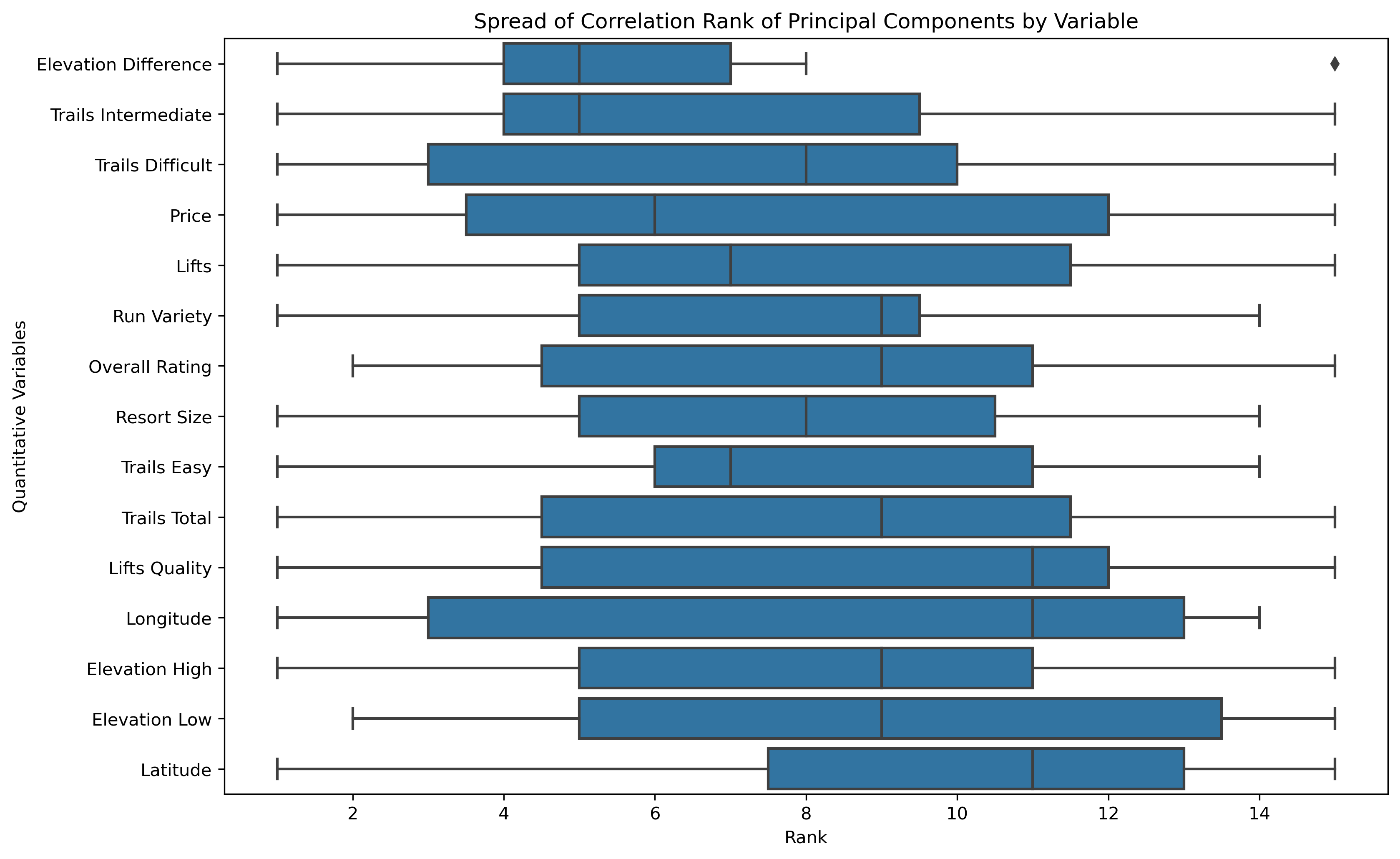
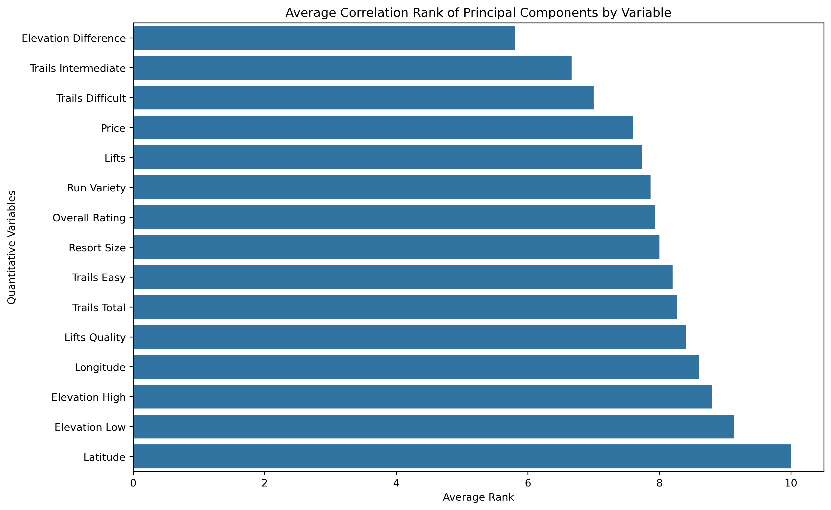
Elevation Difference is commonly the highest influencing original feature, while Latitude is commonly the lowest influencing original feature.
Explained and Cumulative Variance - Table
| principal_components | explained_variance | cumulative_variance |
|---|---|---|
| principal_component_1 | 36.96% | 36.96% |
| principal_component_2 | 14.09% | 51.04% |
| principal_component_3 | 8.91% | 59.95% |
| principal_component_4 | 5.34% | 65.29% |
| principal_component_5 | 4.56% | 69.85% |
| principal_component_6 | 4.45% | 74.31% |
| principal_component_7 | 4.31% | 78.61% |
| principal_component_8 | 4.12% | 82.73% |
| principal_component_9 | 3.89% | 86.63% |
| principal_component_10 | 3.45% | 90.08% |
| principal_component_11 | 3.25% | 93.33% |
| principal_component_12 | 2.61% | 95.94% |
| principal_component_13 | 1.53% | 97.47% |
| principal_component_14 | 1.44% | 98.90% |
| principal_component_15 | 0.52% | 99.43% |
| principal_component_16 | 0.42% | 99.85% |
| principal_component_17 | 0.06% | 99.91% |
| principal_component_18 | 0.04% | 99.95% |
| principal_component_19 | 0.03% | 99.98% |
| principal_component_20 | 0.02% | 100.00% |
| principal_component_21 | 0.00% | 100.00% |
| principal_component_22 | 0.00% | 100.00% |
Explained and Cumulative Variance - Visual
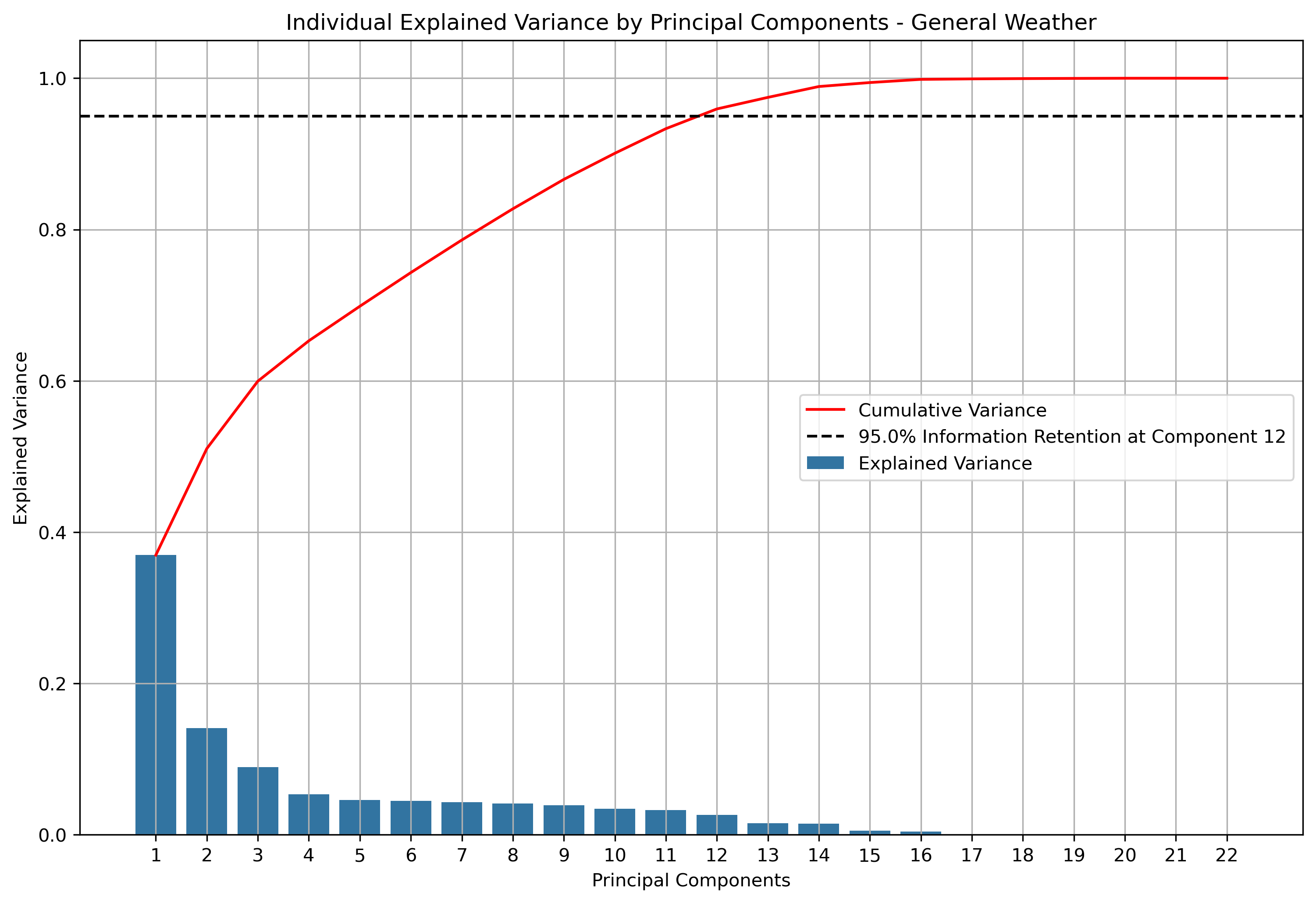
Illustrated above is how much information is retained or explained by each principal component. The principal components are ordered by descending associated eigenvalues, such that the principal component with the largest associated eigenvalue is first. This means that the principal components decreasingly explain the variance in the dataset. For this particular dataset, it takes 12 principal components until 95% of variance within the dataset is explained.
Eigenvalues - Python Output
print(pca.explained_variance_)
Eigenvalues Results:
[8.13046790e+00
 3.09882044e+00
 1.95971060e+00
 1.17444139e+00
 1.00421464e+00
 9.79725935e-01
 9.47683726e-01
 9.06603608e-01
 8.56151879e-01
 7.59333726e-01
 7.15182152e-01
 5.74145340e-01
 3.36380706e-01
 3.15792092e-01
 1.15469316e-01
 9.25721624e-02
 1.40815413e-02
 8.75185242e-03
 5.67468881e-03
 4.04961900e-03
 6.83425476e-04
 9.11417831e-05]
Eigenvalues - Table
| Principal Component | Eigenvalue |
|---|---|
| Principal Component 1 | 8.130468 |
| Principal Component 2 | 3.098820 |
| Principal Component 3 | 1.959711 |
| Principal Component 4 | 1.174441 |
| Principal Component 5 | 1.004215 |
| Principal Component 6 | 0.979726 |
| Principal Component 7 | 0.947684 |
| Principal Component 8 | 0.906604 |
| Principal Component 9 | 0.856152 |
| Principal Component 10 | 0.759334 |
| Principal Component 11 | 0.715182 |
| Principal Component 12 | 0.574145 |
| Principal Component 13 | 0.336381 |
| Principal Component 14 | 0.315792 |
| Principal Component 15 | 0.115469 |
| Principal Component 16 | 0.092572 |
| Principal Component 17 | 0.014082 |
| Principal Component 18 | 0.008752 |
| Principal Component 19 | 0.005675 |
| Principal Component 20 | 0.004050 |
| Principal Component 21 | 0.000683 |
| Principal Component 22 | 0.000091 |
The highest 3 eigenvalues for this dataset are:
- 8.130468
- 3.098820
- 1.95971060
Loadings - Table
| Feature | principal_component_1 | principal_component_2 | principal_component_3 | principal_component_4 | principal_component_5 | principal_component_6 | principal_component_7 | principal_component_8 | principal_component_9 | principal_component_10 | principal_component_11 | principal_component_12 | principal_component_13 | principal_component_14 | principal_component_15 | principal_component_16 | principal_component_17 | principal_component_18 | principal_component_19 | principal_component_20 | principal_component_21 | principal_component_22 |
|---|---|---|---|---|---|---|---|---|---|---|---|---|---|---|---|---|---|---|---|---|---|---|
| tempmax | 0.341702 | 0.044847 | 0.021813 | 0.005786 | -0.018956 | -0.054797 | -0.006958 | 0.020151 | -0.047909 | 0.062773 | 0.095301 | -0.082699 | -0.007336 | -0.024372 | 0.001069 | -0.471893 | 0.142666 | 0.396140 | -0.486184 | -0.350631 | -0.307923 | 0.000344 |
| tempmin | 0.318129 | 0.198307 | 0.062902 | -0.017631 | -0.012820 | -0.014266 | 0.015130 | 0.036999 | -0.067076 | 0.025714 | 0.085684 | 0.060234 | 0.090524 | -0.064892 | -0.010493 | 0.524318 | 0.172907 | 0.586617 | 0.292904 | 0.192406 | -0.229889 | -0.000803 |
| temp | 0.339381 | 0.116827 | 0.046131 | -0.006776 | -0.017000 | -0.035506 | 0.006418 | 0.029500 | -0.057968 | 0.045714 | 0.086429 | -0.021250 | 0.045838 | -0.046324 | -0.030234 | -0.017947 | 0.280062 | -0.040248 | -0.380459 | 0.460633 | 0.640855 | 0.000790 |
| feelslikemax | 0.340382 | 0.061936 | -0.006827 | 0.015381 | -0.018068 | -0.049867 | -0.004156 | 0.025218 | -0.041888 | 0.054500 | 0.098681 | -0.080560 | -0.007052 | 0.002475 | 0.011091 | -0.507938 | -0.342769 | 0.138684 | 0.615191 | 0.007112 | 0.286684 | -0.000257 |
| feelslikemin | 0.322287 | 0.193705 | 0.007469 | -0.005124 | -0.016236 | -0.017912 | 0.023242 | 0.050376 | -0.056063 | 0.027384 | 0.094147 | 0.028906 | 0.091368 | -0.004112 | -0.002443 | 0.432178 | -0.534140 | -0.156861 | -0.220271 | -0.489090 | 0.220190 | 0.001089 |
| feelslike | 0.338886 | 0.123437 | 0.002091 | 0.004709 | -0.018825 | -0.036151 | 0.013941 | 0.040382 | -0.048706 | 0.041159 | 0.092810 | -0.036113 | 0.049999 | -0.001805 | -0.020851 | -0.069669 | -0.288175 | -0.440967 | -0.097094 | 0.501021 | -0.553790 | -0.001347 |
| dew | 0.287168 | 0.297378 | -0.004698 | 0.005349 | 0.002762 | 0.040080 | 0.026739 | 0.051906 | -0.027620 | -0.024594 | 0.040776 | 0.199286 | -0.233186 | 0.008548 | 0.006854 | -0.005293 | 0.565545 | -0.463263 | 0.276239 | -0.335317 | -0.059652 | 0.000183 |
| humidity | -0.122013 | 0.419951 | -0.115953 | 0.048419 | 0.036596 | 0.145030 | 0.042465 | 0.062597 | 0.079071 | -0.156794 | -0.132779 | 0.451269 | -0.587302 | 0.118840 | -0.005816 | -0.086203 | -0.241926 | 0.208159 | -0.140874 | 0.154519 | 0.025833 | 0.000040 |
| precip | -0.010098 | 0.215811 | 0.161635 | 0.191367 | -0.025211 | -0.182404 | 0.041496 | -0.254172 | 0.862951 | 0.097955 | 0.141329 | -0.108259 | 0.026239 | -0.058726 | 0.009745 | 0.008778 | 0.006038 | -0.003970 | 0.001252 | -0.002889 | -0.000160 | -0.000068 |
| snow | -0.082881 | 0.044502 | 0.166281 | 0.555183 | 0.021724 | 0.193211 | 0.245988 | 0.186686 | -0.128819 | 0.682821 | -0.195302 | 0.000216 | -0.014353 | -0.027384 | 0.011940 | 0.001601 | -0.001360 | -0.003134 | 0.003109 | -0.002063 | -0.000728 | -0.000075 |
| snowdepth | -0.108000 | -0.089923 | 0.114606 | 0.538328 | -0.007242 | 0.072542 | 0.259089 | 0.119135 | -0.128847 | -0.480026 | 0.580657 | -0.020350 | -0.020873 | -0.070036 | -0.026394 | -0.002854 | 0.004371 | 0.001916 | -0.003272 | 0.000855 | 0.001137 | -0.000190 |
| windgust | -0.037873 | -0.041897 | 0.608182 | -0.114671 | -0.041556 | -0.125841 | -0.008027 | -0.143867 | -0.111278 | 0.072721 | 0.147746 | 0.166057 | 0.008198 | 0.712664 | -0.016480 | -0.010417 | -0.003311 | 0.003304 | -0.000480 | 0.004002 | 0.000010 | -0.000049 |
| windspeed | -0.036032 | -0.118269 | 0.585353 | -0.165278 | -0.003624 | -0.073614 | -0.082994 | -0.180094 | -0.127973 | 0.046940 | 0.025757 | 0.221513 | -0.224230 | -0.665490 | -0.010867 | -0.026344 | -0.082005 | -0.030418 | -0.002297 | -0.006013 | -0.005779 | -0.000032 |
| winddir | 0.006041 | -0.118088 | 0.183010 | -0.275912 | 0.196100 | 0.517622 | -0.201720 | 0.605307 | 0.314999 | 0.070962 | 0.236307 | 0.021670 | 0.040003 | 0.002268 | -0.016892 | -0.020157 | -0.006732 | 0.002559 | -0.001067 | 0.001510 | -0.000121 | 0.000050 |
| pressure | -0.042439 | -0.242871 | -0.367211 | 0.022711 | -0.056056 | -0.195316 | -0.175803 | -0.061895 | 0.031802 | 0.353732 | 0.442780 | 0.622535 | 0.128541 | -0.022079 | -0.023386 | -0.020238 | 0.003018 | 0.002503 | -0.005864 | 0.008070 | 0.001391 | 0.000036 |
| cloudcover | -0.143978 | 0.378492 | 0.112290 | -0.039500 | 0.008244 | 0.151272 | 0.177593 | -0.013583 | -0.018102 | -0.185363 | -0.178741 | 0.382045 | 0.705924 | -0.106654 | 0.057148 | -0.203331 | 0.006354 | -0.004464 | -0.003010 | -0.013794 | -0.001576 | 0.000002 |
| visibility | 0.033442 | -0.092879 | -0.127334 | -0.370916 | 0.014443 | 0.405082 | 0.666985 | -0.381592 | 0.014957 | 0.155139 | 0.218838 | -0.043098 | -0.084986 | 0.000620 | 0.013974 | 0.006795 | -0.006164 | 0.009205 | -0.003111 | 0.006587 | 0.001185 | 0.000173 |
| solarradiation | 0.249173 | -0.328804 | 0.026208 | 0.126705 | 0.013849 | 0.075671 | 0.095815 | -0.028176 | 0.146790 | -0.146259 | -0.266039 | 0.197221 | 0.021070 | 0.039869 | -0.376854 | 0.015129 | -0.007404 | 0.002499 | 0.008437 | -0.010344 | -0.002550 | 0.707127 |
| solarenergy | 0.249208 | -0.328749 | 0.026024 | 0.126423 | 0.014036 | 0.075869 | 0.095797 | -0.028325 | 0.146781 | -0.146174 | -0.266113 | 0.197316 | 0.020988 | 0.039898 | -0.376936 | 0.015259 | -0.007235 | 0.002425 | 0.007129 | -0.012008 | -0.000448 | -0.707083 |
| uvindex | 0.247059 | -0.324512 | 0.031381 | 0.125097 | 0.018864 | 0.065207 | 0.045536 | -0.019337 | 0.118343 | -0.132217 | -0.184556 | 0.176461 | -0.023376 | 0.045838 | 0.841558 | 0.037803 | -0.006514 | -0.000388 | -0.017060 | 0.025291 | 0.003072 | -0.000063 |
| moonphase | 0.002742 | 0.000063 | -0.015324 | -0.026925 | 0.931048 | -0.316603 | 0.171830 | 0.030751 | -0.028583 | 0.010762 | 0.000803 | 0.021752 | 0.006781 | 0.004540 | 0.000149 | -0.000737 | -0.000141 | -0.000184 | -0.000295 | 0.000224 | 0.000180 | 0.000083 |
| severerisk | 0.068095 | 0.070250 | -0.026231 | 0.240096 | 0.290736 | 0.512476 | -0.511994 | -0.547921 | -0.101090 | -0.002029 | 0.066625 | -0.055125 | 0.051231 | 0.042252 | -0.019849 | 0.002587 | -0.005343 | -0.002315 | -0.005448 | 0.001603 | -0.001470 | 0.000128 |
Loadings - Barplot
Loadings - Boxplot
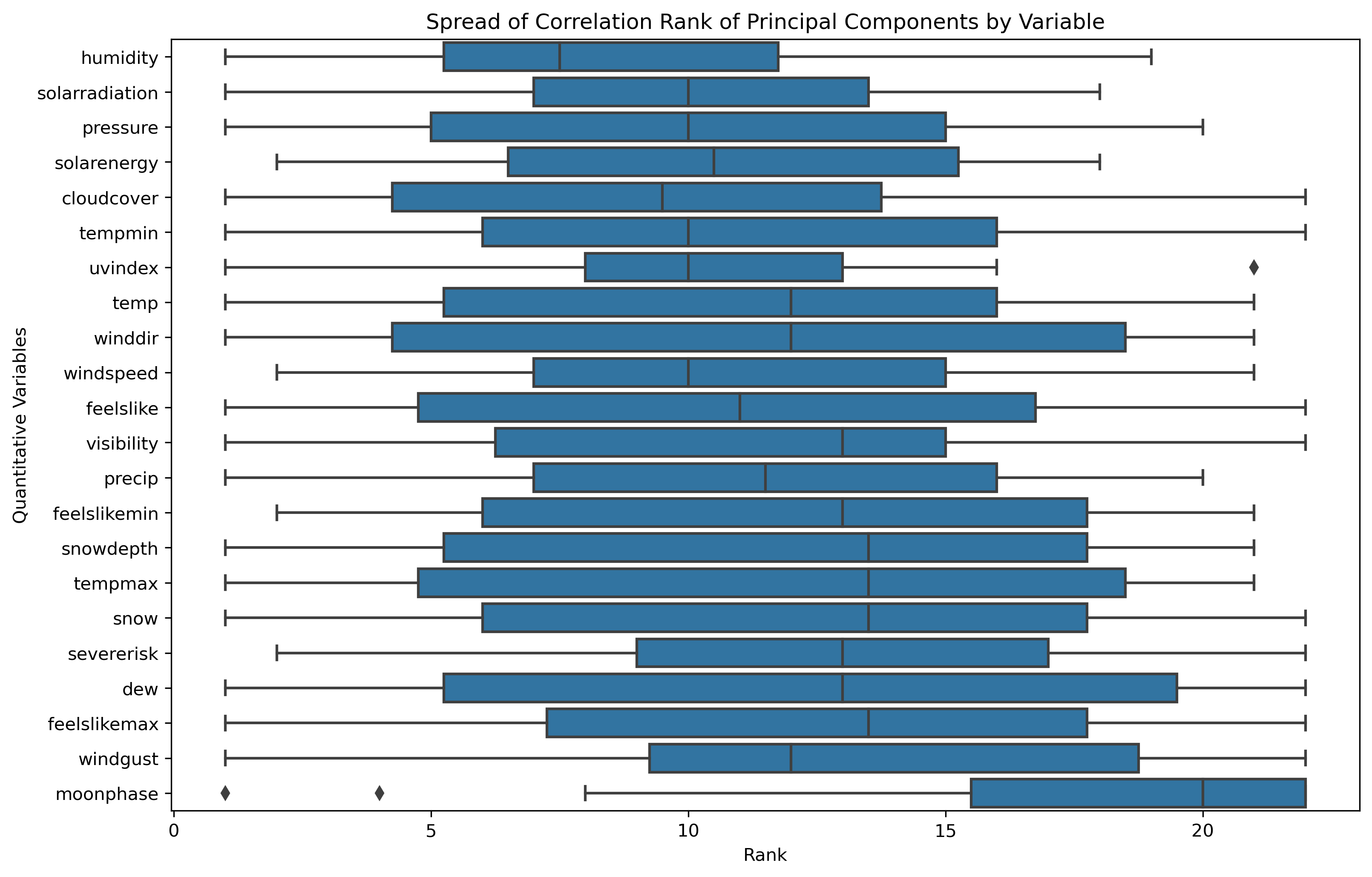
Humidity is commonly the highest influencing original feature, while Moonphase is commonly the lowest influencing original feature.
Explained and Cumulative Variance - Table
| principal_components | explained_variance | cumulative_variance |
|---|---|---|
| principal_component_1 | 33.12% | 33.12% |
| principal_component_2 | 28.13% | 61.25% |
| principal_component_3 | 21.87% | 83.12% |
| principal_component_4 | 16.88% | 100.00% |
Explained and Cumulative Variance - Visual
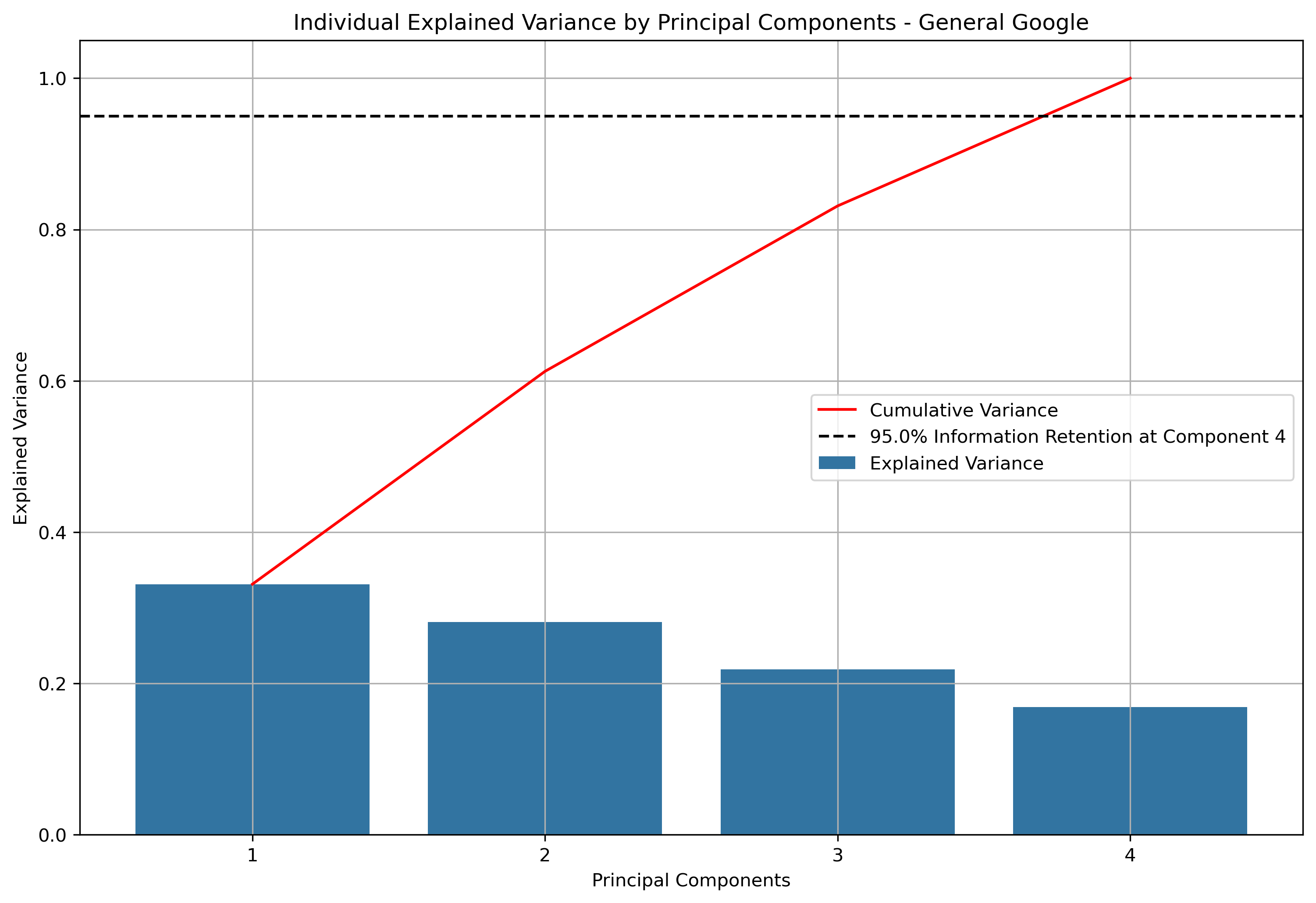
Illustrated above is how much information is retained or explained by each principal component. The principal components are ordered by descending associated eigenvalues, such that the principal component with the largest associated eigenvalue is first. This means that the principal components decreasingly explain the variance in the dataset. For this particular dataset, it takes all 4 principal components until 95% of variance within the dataset is explained.
Eigenvalues - Python Output
print(pca.explained_variance_)
Eigenvalues Results:
[1.32498375
 1.1252785
 0.87469825
 0.6752141]
Eigenvalues - Table
| Principal Component | Eigenvalue |
|---|---|
| Principal Component 1 | 1.324984 |
| Principal Component 2 | 1.125278 |
| Principal Component 3 | 0.874698 |
| Principal Component 4 | 0.675214 |
The highest 3 eigenvalues for this dataset are:
- 1.32498375
- 1.1252785
- 0.87469825
Loadings - Table
| Feature | principal_component_1 | principal_component_2 | principal_component_3 | principal_component_4 |
|---|---|---|---|---|
| Latitude | 0.704954 | 0.054736 | 0.053544 | 0.705108 |
| Longitude | -0.693377 | -0.133590 | 0.148636 | 0.692308 |
| rating | -0.046771 | 0.706612 | 0.703370 | -0.061504 |
| total_ratings | -0.141710 | 0.692717 | -0.693045 | 0.140534 |
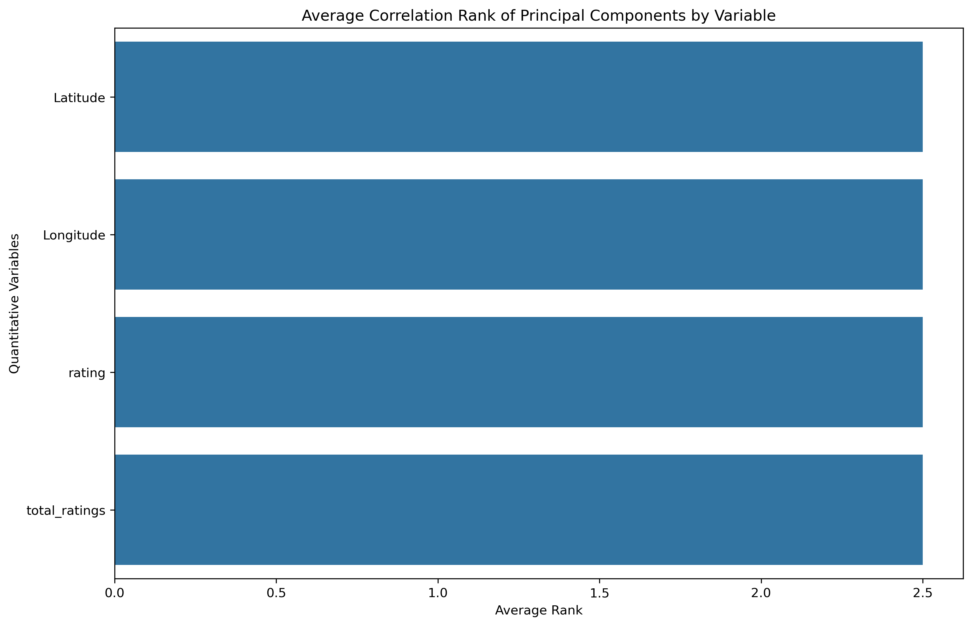
Loadings - Barplot
Loadings - Boxplot
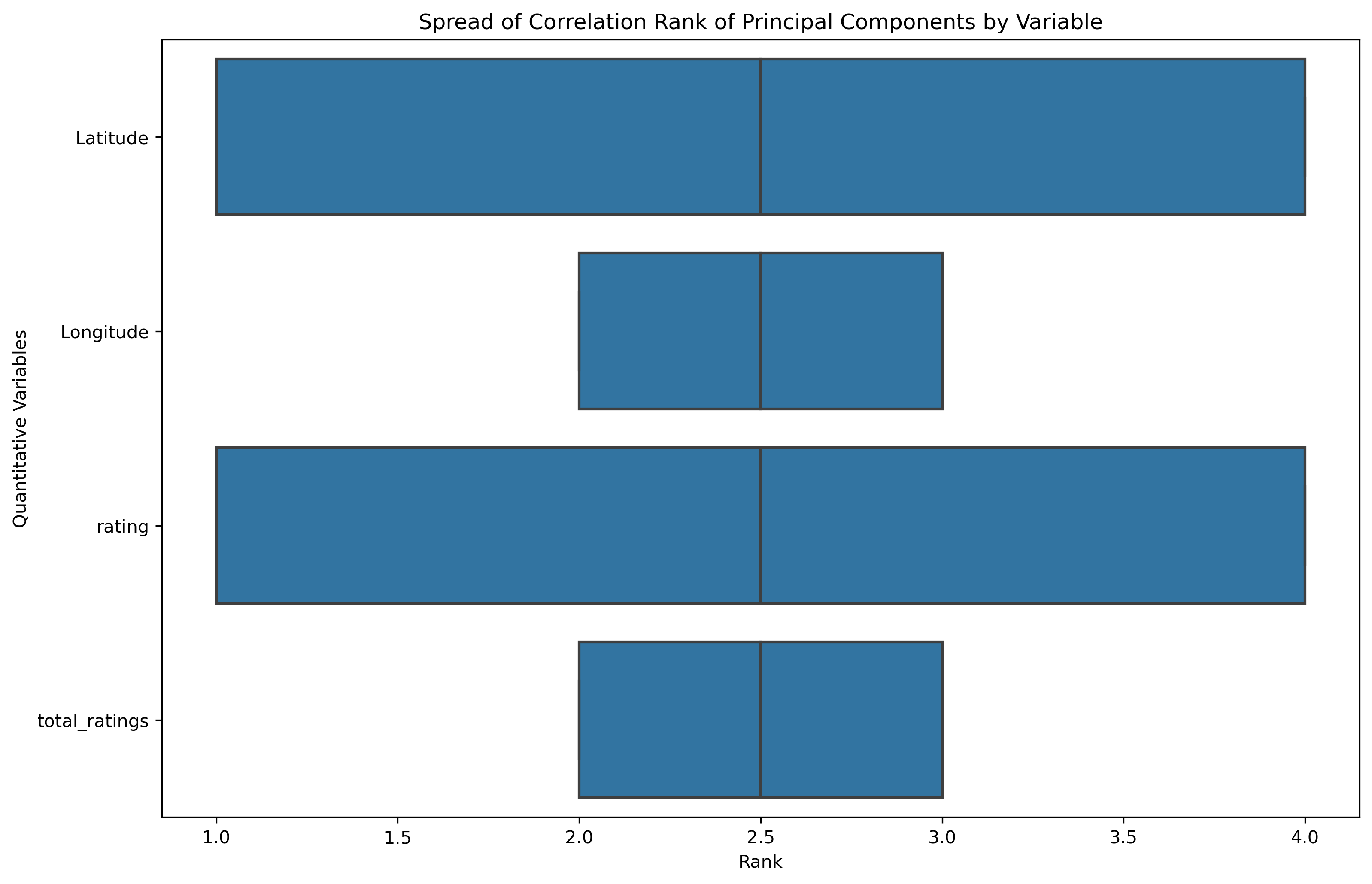
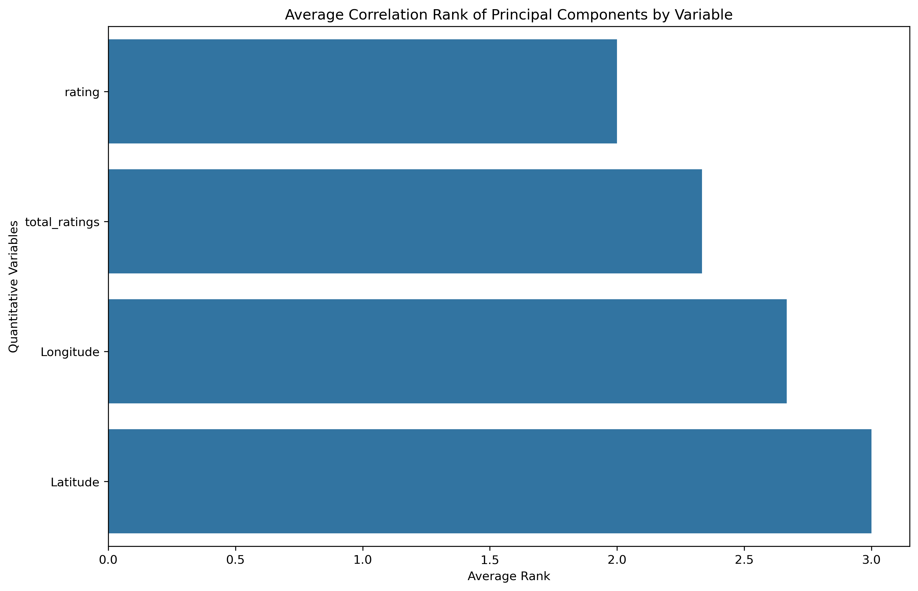
Each of the original features have equivalent average influence on the principal components. However, Latitude and Rating have a smaller ranking spread than Longitude and Total Ratings.
Explained and Cumulative Variance - Table
| principal_components | explained_variance | cumulative_variance |
|---|---|---|
| principal_component_1 | 67.37% | 67.37% |
| principal_component_2 | 9.88% | 77.25% |
| principal_component_3 | 8.37% | 85.63% |
Explained and Cumulative Variance - Visual
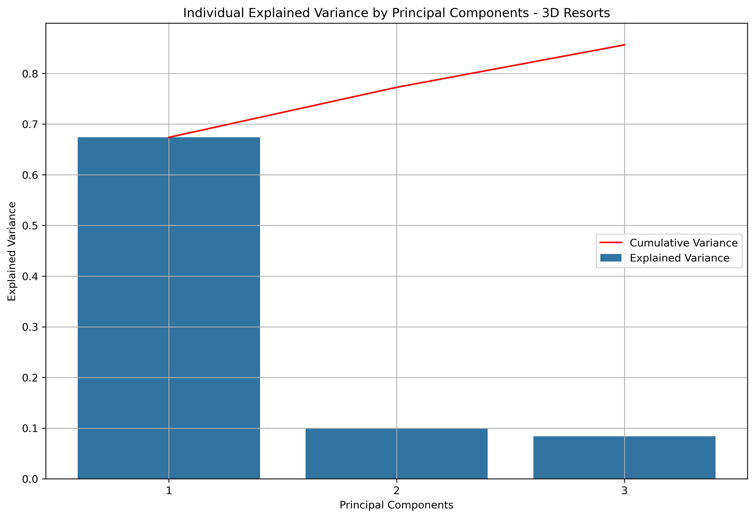
For three dimensional principal component analysis, 85.63% of information is retained from the original data.
Loadings - Table
| Feature | principal_component_1 | principal_component_2 | principal_component_3 |
|---|---|---|---|
| Overall Rating | 0.295563 | 0.128409 | 0.070401 |
| Elevation Difference | 0.286191 | 0.006434 | 0.127605 |
| Elevation Low | 0.217565 | -0.531208 | -0.238126 |
| Elevation High | 0.259075 | -0.424419 | -0.153443 |
| Trails Total | 0.300028 | 0.106896 | 0.083704 |
| Trails Easy | 0.262651 | 0.127329 | 0.075640 |
| Trails Intermediate | 0.289896 | 0.097366 | 0.072066 |
| Trails Difficult | 0.276246 | 0.087010 | 0.084746 |
| Lifts | 0.251273 | 0.201499 | -0.109092 |
| Price | 0.289004 | 0.059050 | -0.112851 |
| Resort Size | 0.298762 | 0.081368 | 0.076491 |
| Run Variety | 0.296819 | 0.045266 | 0.091947 |
| Lifts Quality | 0.215449 | 0.227293 | -0.101905 |
| Latitude | -0.082354 | 0.010183 | 0.845442 |
| Longitude | -0.140384 | 0.609871 | -0.330620 |
Loadings - Barplot
Loadings - Boxplot
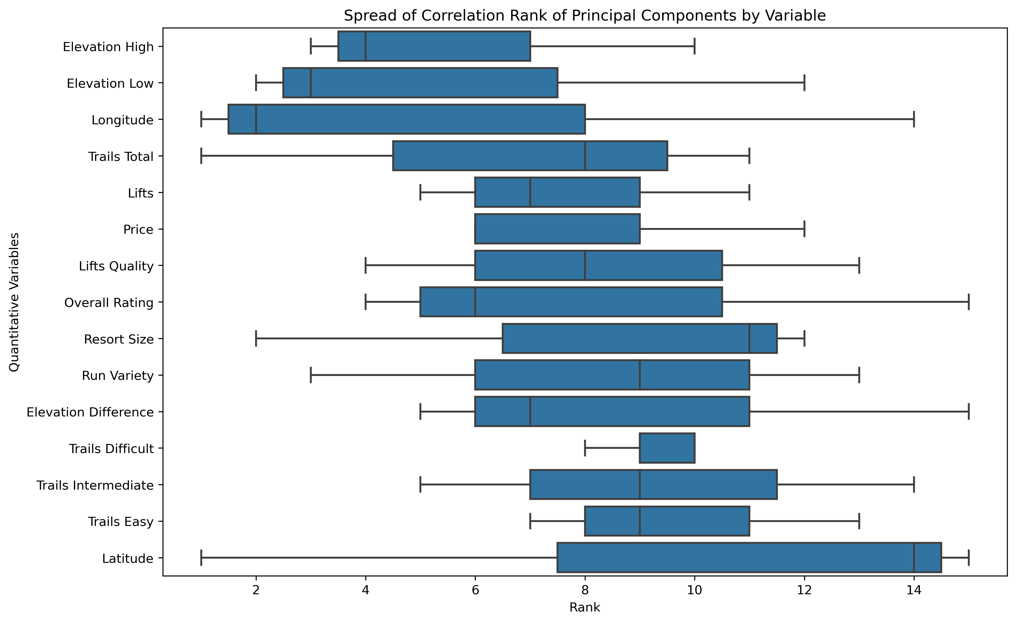
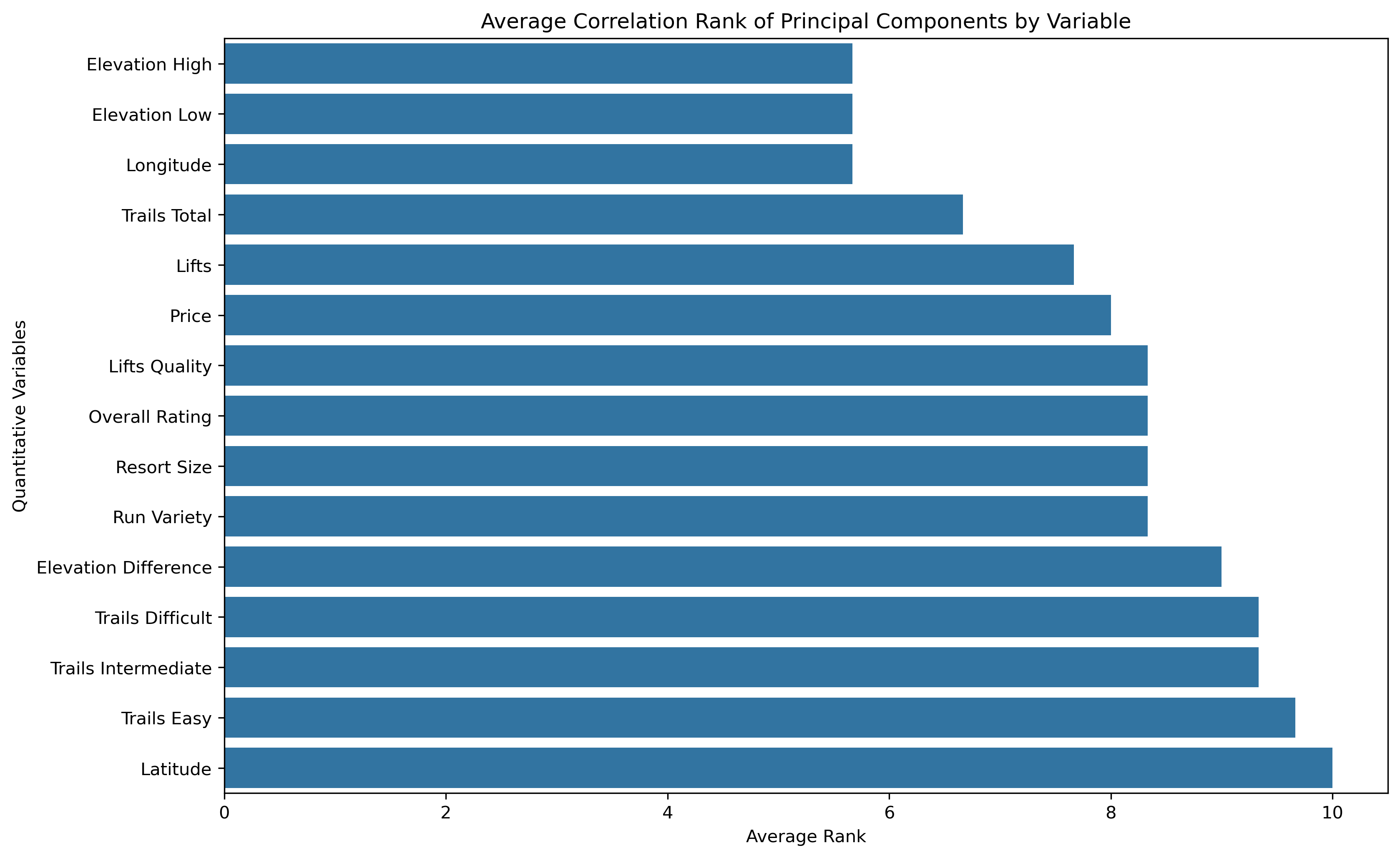
The loadings matrix differs between the full dimensional PCA and the three dimensional PCA.
Visualizing PCA in 3 Dimensions with Labels
Several different labels were applied to the data projected into the PCA space. Some interesting clusters can be observed using this. Note that the labels can be toggled through the legend.Resorts with Country Label - Expand Image
Resorts with Region Label - Expand Image
Resorts with Pass Label - Expand Image
Explained and Cumulative Variance - Table
| principal_components | explained_variance | cumulative_variance |
|---|---|---|
| principal_component_1 | 36.96% | 36.96% |
| principal_component_2 | 14.09% | 51.04% |
| principal_component_3 | 8.91% | 59.95% |
Explained and Cumulative Variance - Visual
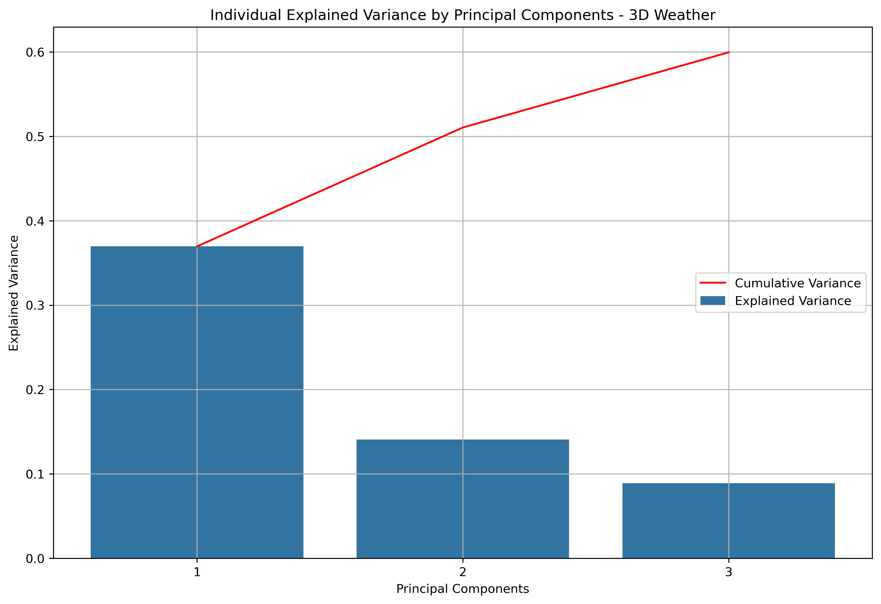
For three dimensional principal component analysis, 59.95% of information is retained from the original data.
Loadings - Table
| Feature | principal_component_1 | principal_component_2 | principal_component_3 |
|---|---|---|---|
| tempmax | 0.341702 | 0.044847 | 0.021813 |
| tempmin | 0.318129 | 0.198307 | 0.062902 |
| temp | 0.339381 | 0.116827 | 0.046131 |
| feelslikemax | 0.340382 | 0.061936 | -0.006827 |
| feelslikemin | 0.322287 | 0.193705 | 0.007469 |
| feelslike | 0.338886 | 0.123437 | 0.002091 |
| dew | 0.287168 | 0.297378 | -0.004698 |
| humidity | -0.122013 | 0.419951 | -0.115953 |
| precip | -0.010098 | 0.215811 | 0.161635 |
| snow | -0.082881 | 0.044502 | 0.166281 |
| snowdepth | -0.108000 | -0.089923 | 0.114606 |
| windgust | -0.037873 | -0.041897 | 0.608182 |
| windspeed | -0.036032 | -0.118269 | 0.585353 |
| winddir | 0.006041 | -0.118088 | 0.183010 |
| pressure | -0.042439 | -0.242871 | -0.367211 |
| cloudcover | -0.143978 | 0.378492 | 0.112290 |
| visibility | 0.033442 | -0.092879 | -0.127334 |
| solarradiation | 0.249173 | -0.328804 | 0.026208 |
| solarenergy | 0.249208 | -0.328749 | 0.026024 |
| uvindex | 0.247059 | -0.324512 | 0.031381 |
| moonphase | 0.002742 | 0.000063 | -0.015324 |
| severerisk | 0.068095 | 0.070250 | -0.026231 |
Loadings - Barplot
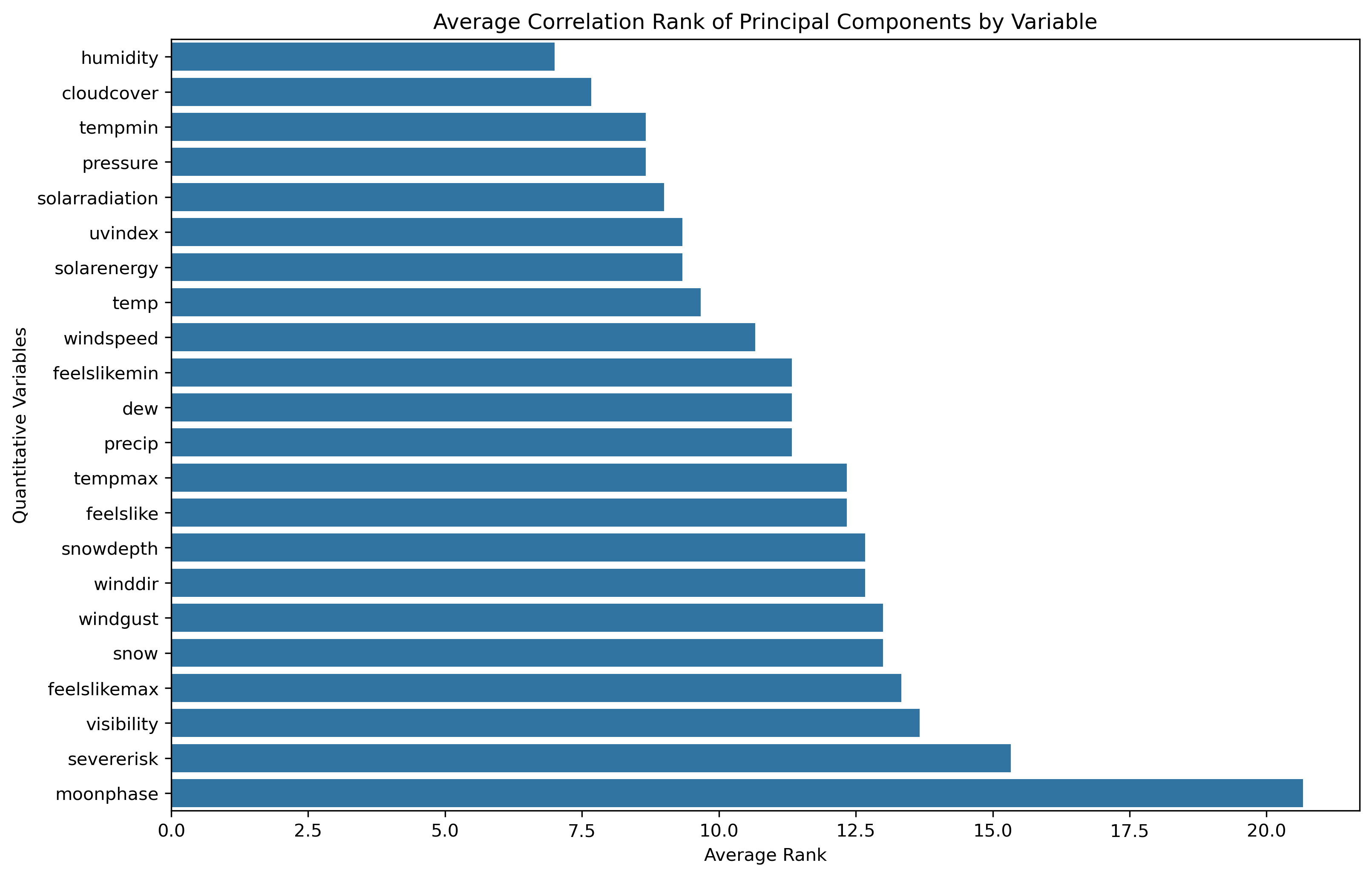
Loadings - Boxplot
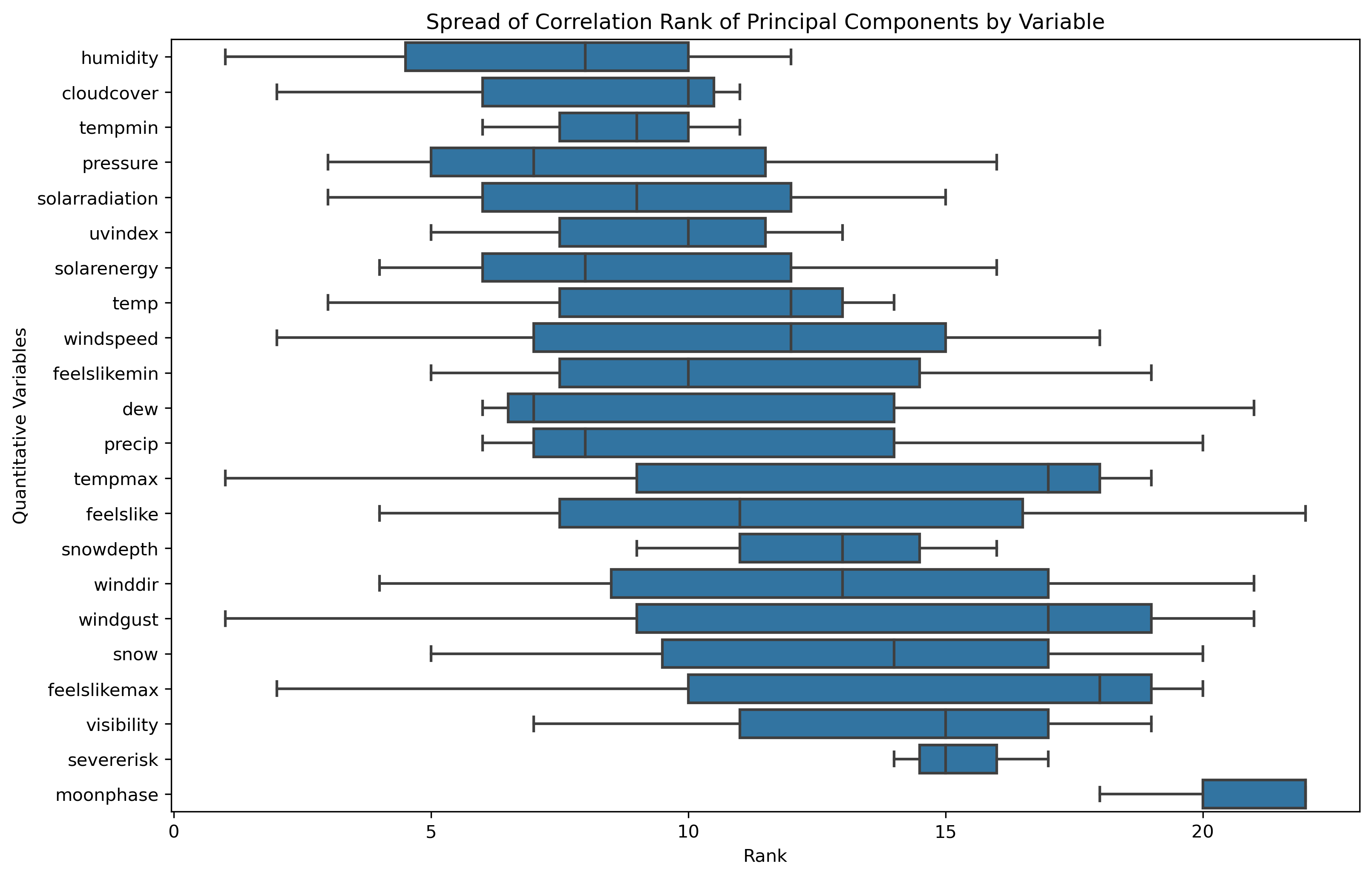
The loadings matrix differs between the full dimensional PCA and the three dimensional PCA.
Visualizing PCA in 3 Dimensions with Labels
The label of weather type was applied to the data projected into the PCA space. Some interesting clusters can be observed using this. Since the weather data is so numerous, a subset aggregated into monthly averages was used for illustrative purposes.Weather Data with Type of Weather Label - Expand Image
Explained and Cumulative Variance - Table
| principal_components | explained_variance | cumulative_variance |
|---|---|---|
| principal_component_1 | 33.12% | 33.12% |
| principal_component_2 | 28.13% | 61.25% |
| principal_component_3 | 21.87% | 83.12% |
Explained and Cumulative Variance - Visual
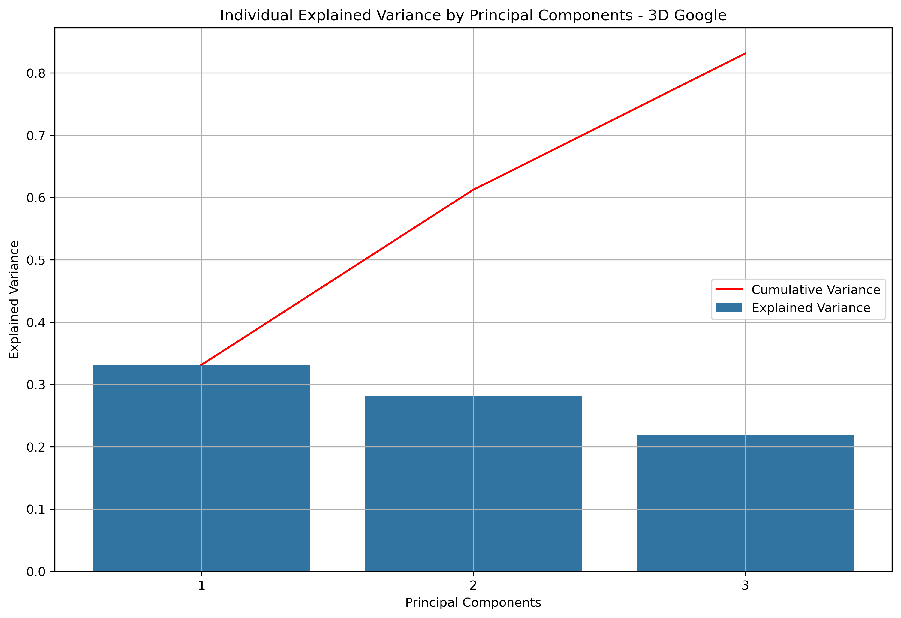
For three dimensional principal component analysis, 83.12% of information is retained from the original data.
Loadings - Table
| Feature | principal_component_1 | principal_component_2 | principal_component_3 |
|---|---|---|---|
| Latitude | 0.704954 | 0.054736 | 0.053544 |
| Longitude | -0.693377 | -0.133590 | 0.148636 |
| rating | -0.046771 | 0.706612 | 0.703370 |
| total_ratings | -0.141710 | 0.692717 | -0.693045 |
Loadings - Barplot
Loadings - Boxplot
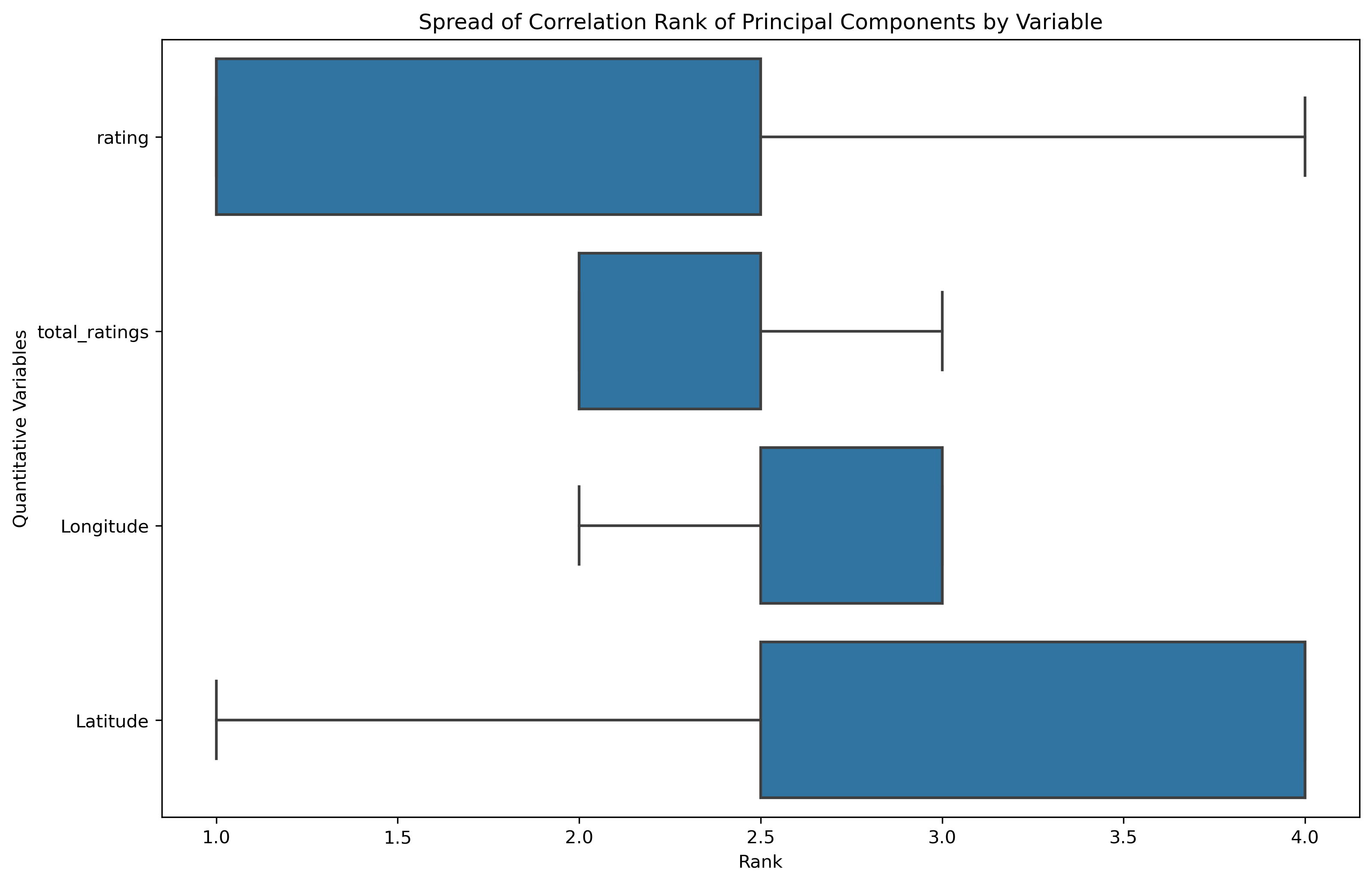
The loadings matrix differs between the full dimensional PCA and the three dimensional PCA.
Visualizing PCA in 3 Dimensions with Labels
A categorical label was applied to the data projected into the PCA space. Some interesting clusters can be observed using this. Since the business data is so numerous, a subset was used for illustrative purposes.Google Places with Business Category Label - Expand Image
Explained and Cumulative Variance - Table
| principal_components | explained_variance | cumulative_variance |
|---|---|---|
| principal_component_1 | 67.37% | 67.37% |
| principal_component_2 | 9.88% | 77.25% |
Explained and Cumulative Variance - Visual
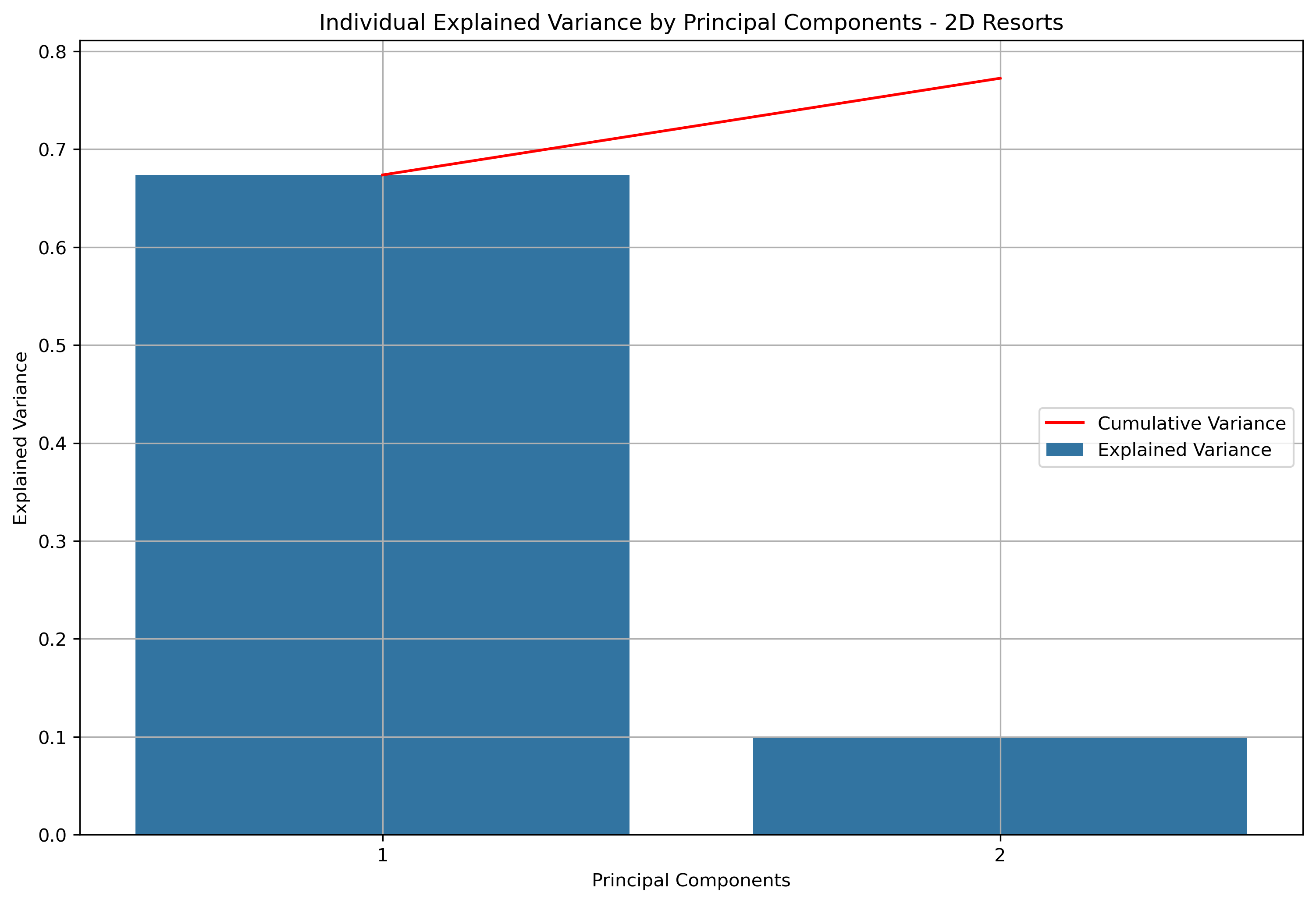
For two dimensional principal component analysis, 77.25% of information is retained from the original data.
Loadings - Table
| Feature | principal_component_1 | principal_component_2 |
|---|---|---|
| Overall Rating | 0.295563 | 0.128409 |
| Elevation Difference | 0.286191 | 0.006434 |
| Elevation Low | 0.217565 | -0.531208 |
| Elevation High | 0.259075 | -0.424419 |
| Trails Total | 0.300028 | 0.106896 |
| Trails Easy | 0.262651 | 0.127329 |
| Trails Intermediate | 0.289896 | 0.097366 |
| Trails Difficult | 0.276246 | 0.087010 |
| Lifts | 0.251273 | 0.201499 |
| Price | 0.289004 | 0.059050 |
| Resort Size | 0.298762 | 0.081368 |
| Run Variety | 0.296819 | 0.045266 |
| Lifts Quality | 0.215449 | 0.227293 |
| Latitude | -0.082354 | 0.010183 |
| Longitude | -0.140384 | 0.609871 |
Loadings - Barplot
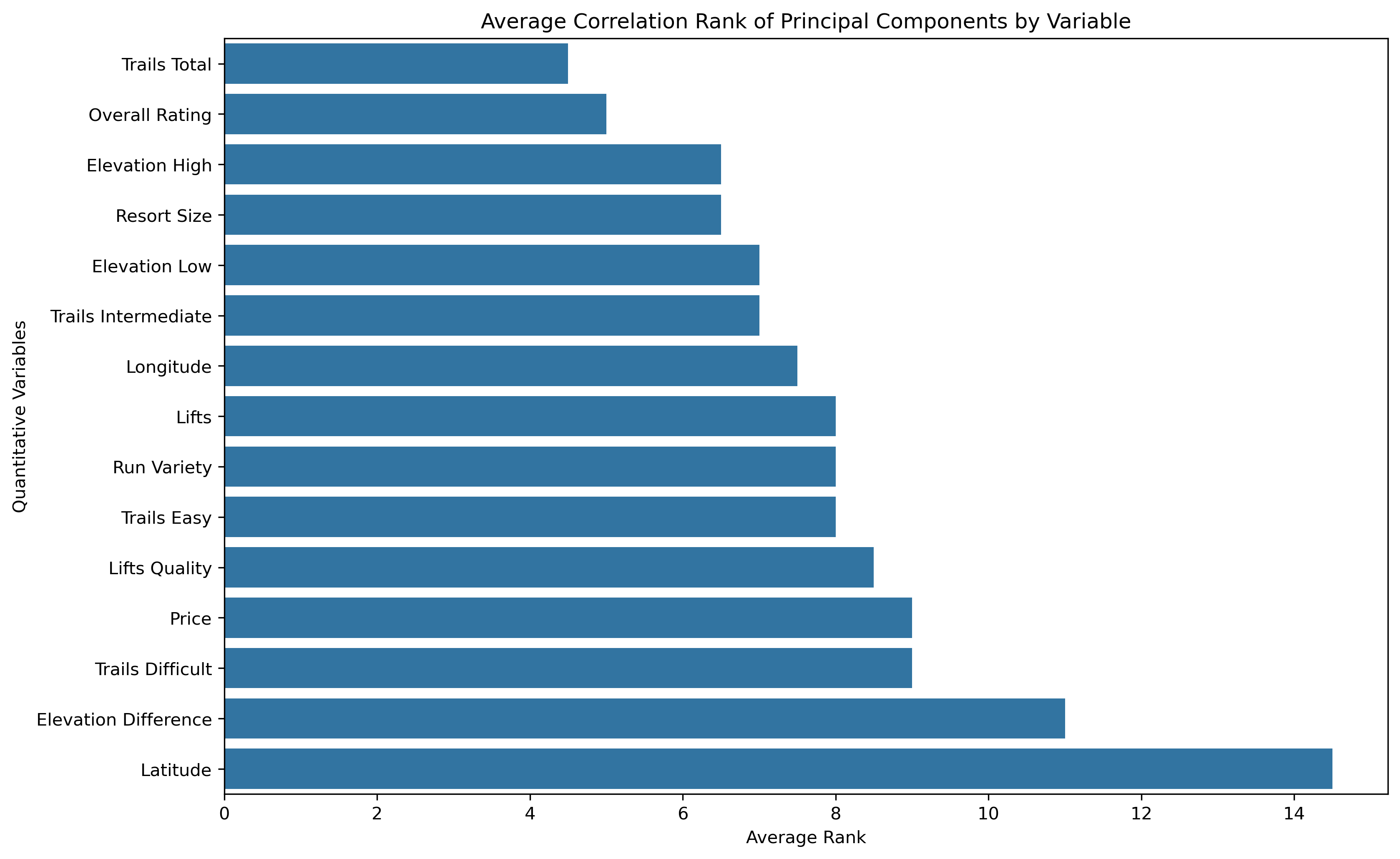
Loadings - Boxplot
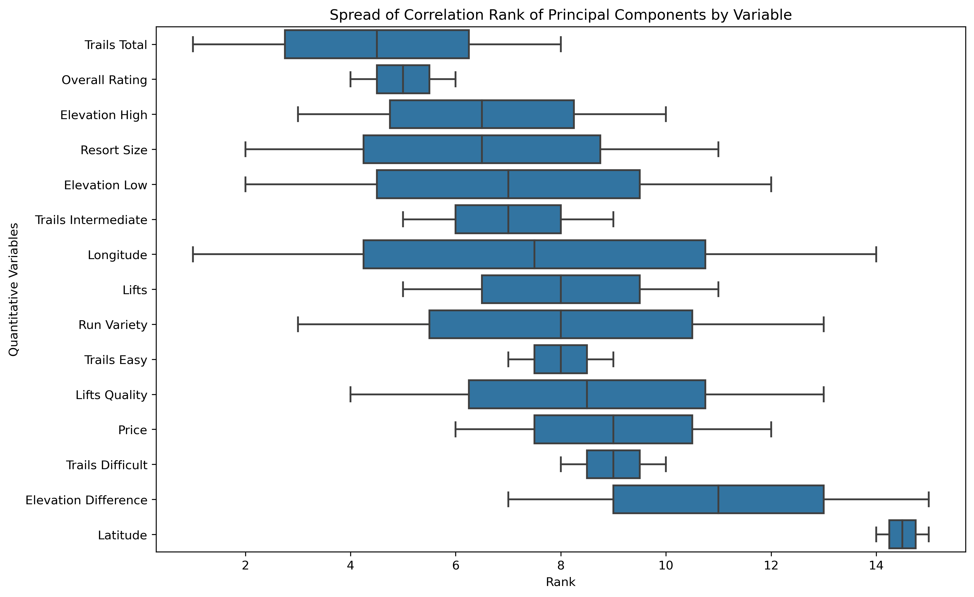
Again, the loadings matrix for two dimensional PCA shows different influence across the original data features.
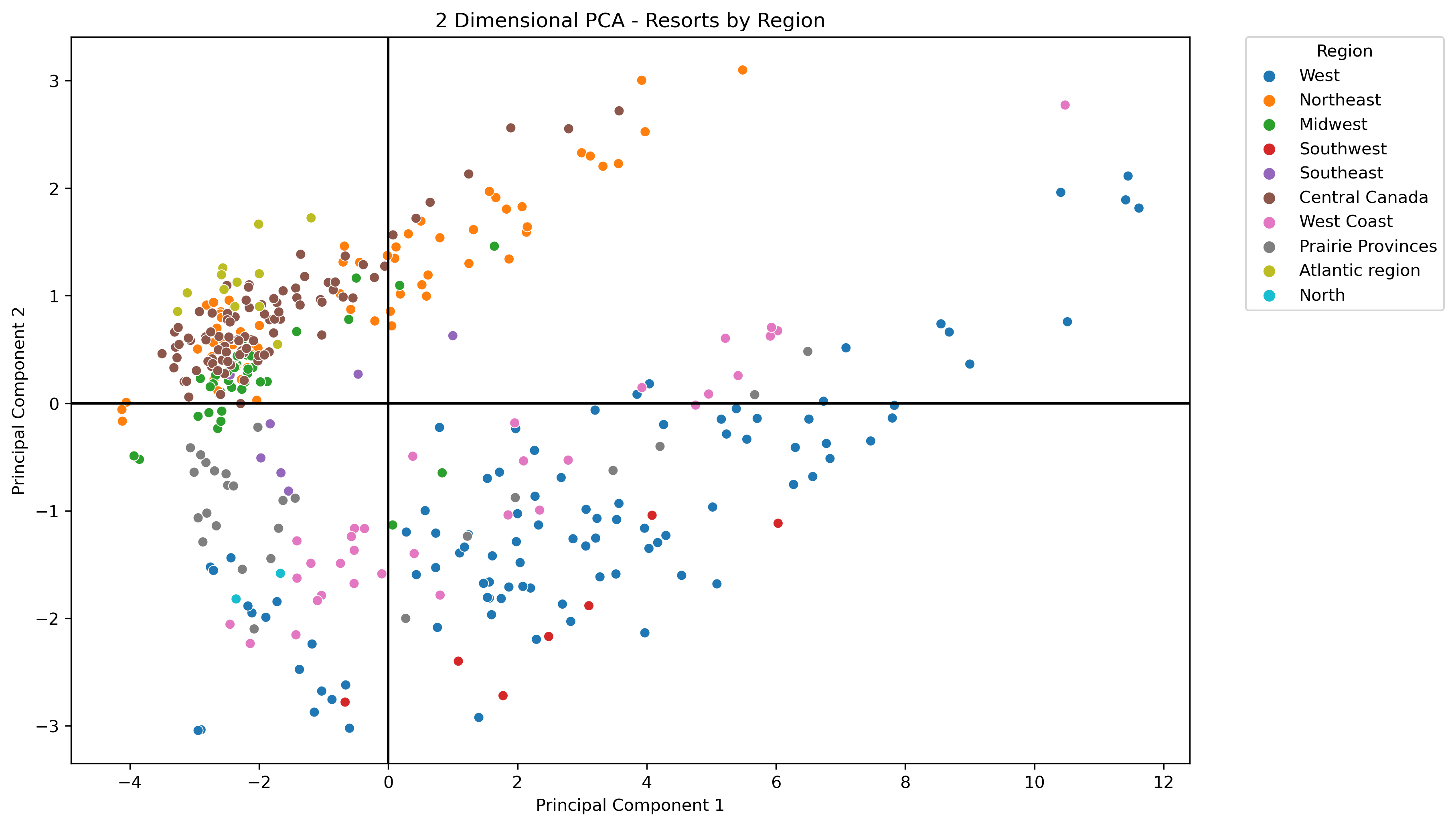
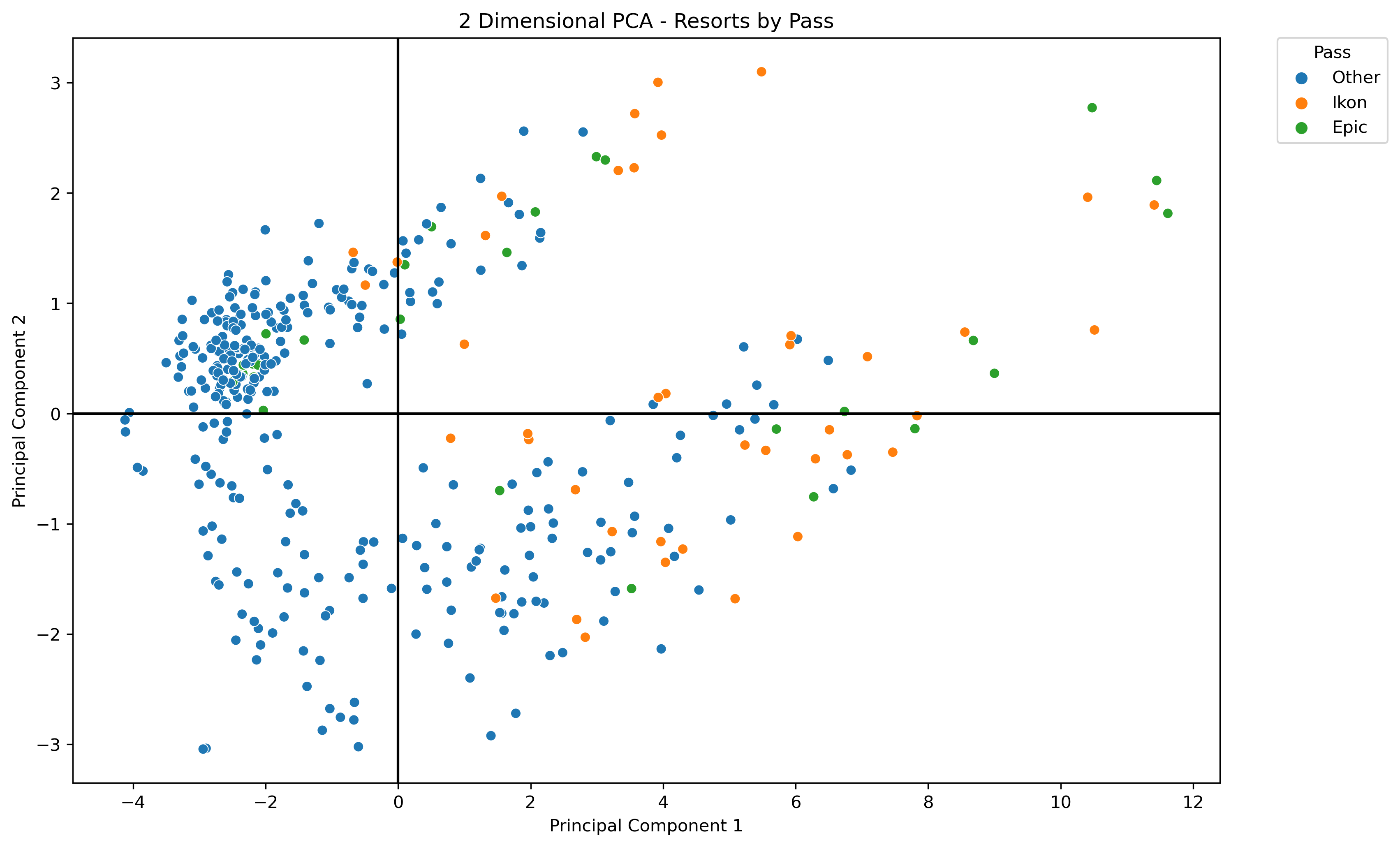
Visualizing PCA in 2 Dimensions with Labels
Several different labels were applied to the data projected into the PCA space. Some interesting patterns can be observed using this.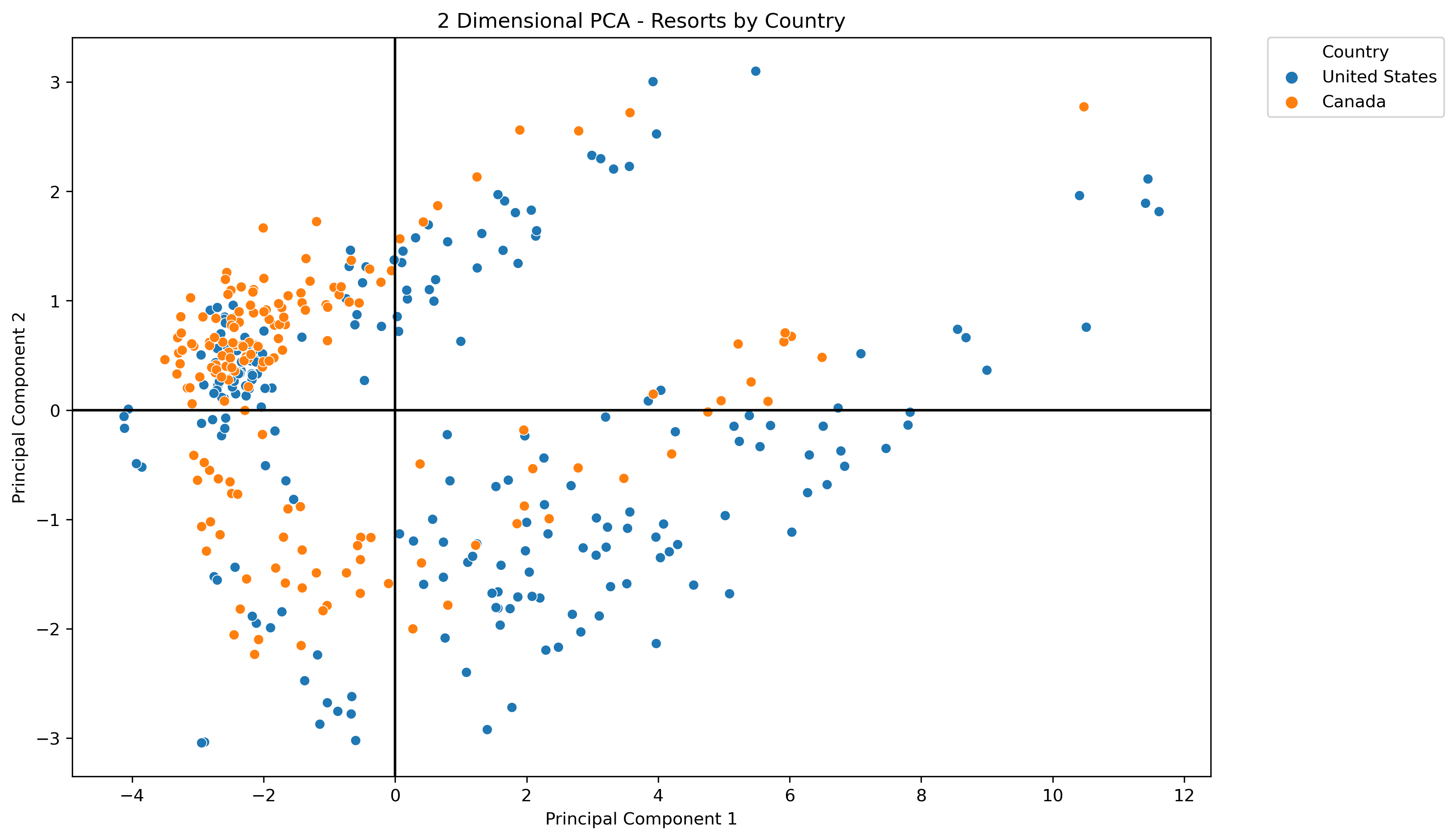
Explained and Cumulative Variance - Table
| principal_components | explained_variance | cumulative_variance |
|---|---|---|
| principal_component_1 | 36.96% | 36.96% |
| principal_component_2 | 14.09% | 51.04% |
Explained and Cumulative Variance - Visual
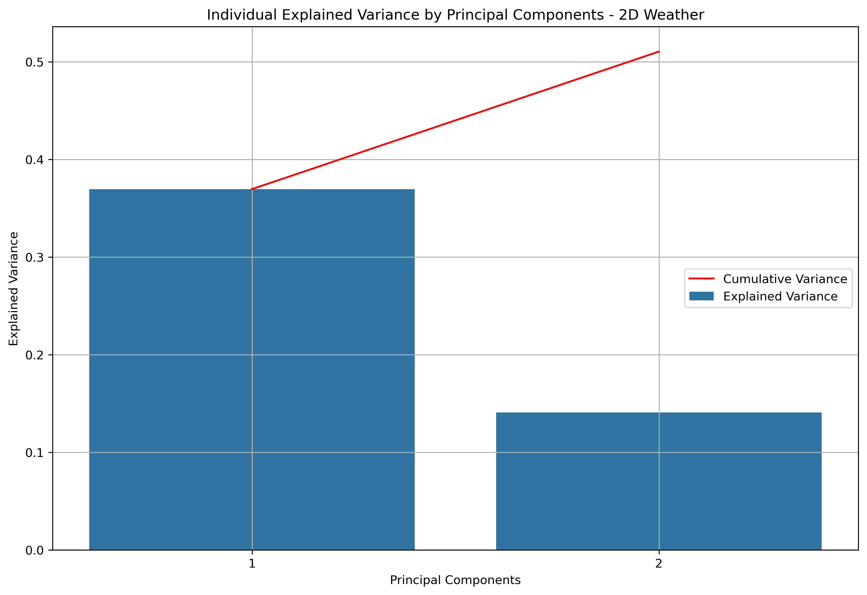
For two dimensional principal component analysis, 51.04% of information is retained from the original data.
Loadings - Table
| Feature | principal_component_1 | principal_component_2 |
|---|---|---|
| tempmax | 0.341702 | 0.044847 |
| tempmin | 0.318129 | 0.198307 |
| temp | 0.339381 | 0.116827 |
| feelslikemax | 0.340382 | 0.061936 |
| feelslikemin | 0.322287 | 0.193705 |
| feelslike | 0.338886 | 0.123437 |
| dew | 0.287168 | 0.297378 |
| humidity | -0.122013 | 0.419951 |
| precip | -0.010098 | 0.215811 |
| snow | -0.082881 | 0.044502 |
| snowdepth | -0.108000 | -0.089923 |
| windgust | -0.037873 | -0.041897 |
| windspeed | -0.036032 | -0.118269 |
| winddir | 0.006041 | -0.118088 |
| pressure | -0.042439 | -0.242871 |
| cloudcover | -0.143978 | 0.378492 |
| visibility | 0.033442 | -0.092879 |
| solarradiation | 0.249173 | -0.328804 |
| solarenergy | 0.249208 | -0.328749 |
| uvindex | 0.247059 | -0.324512 |
| moonphase | 0.002742 | 0.000063 |
| severerisk | 0.068095 | 0.070250 |
Loadings - Barplot
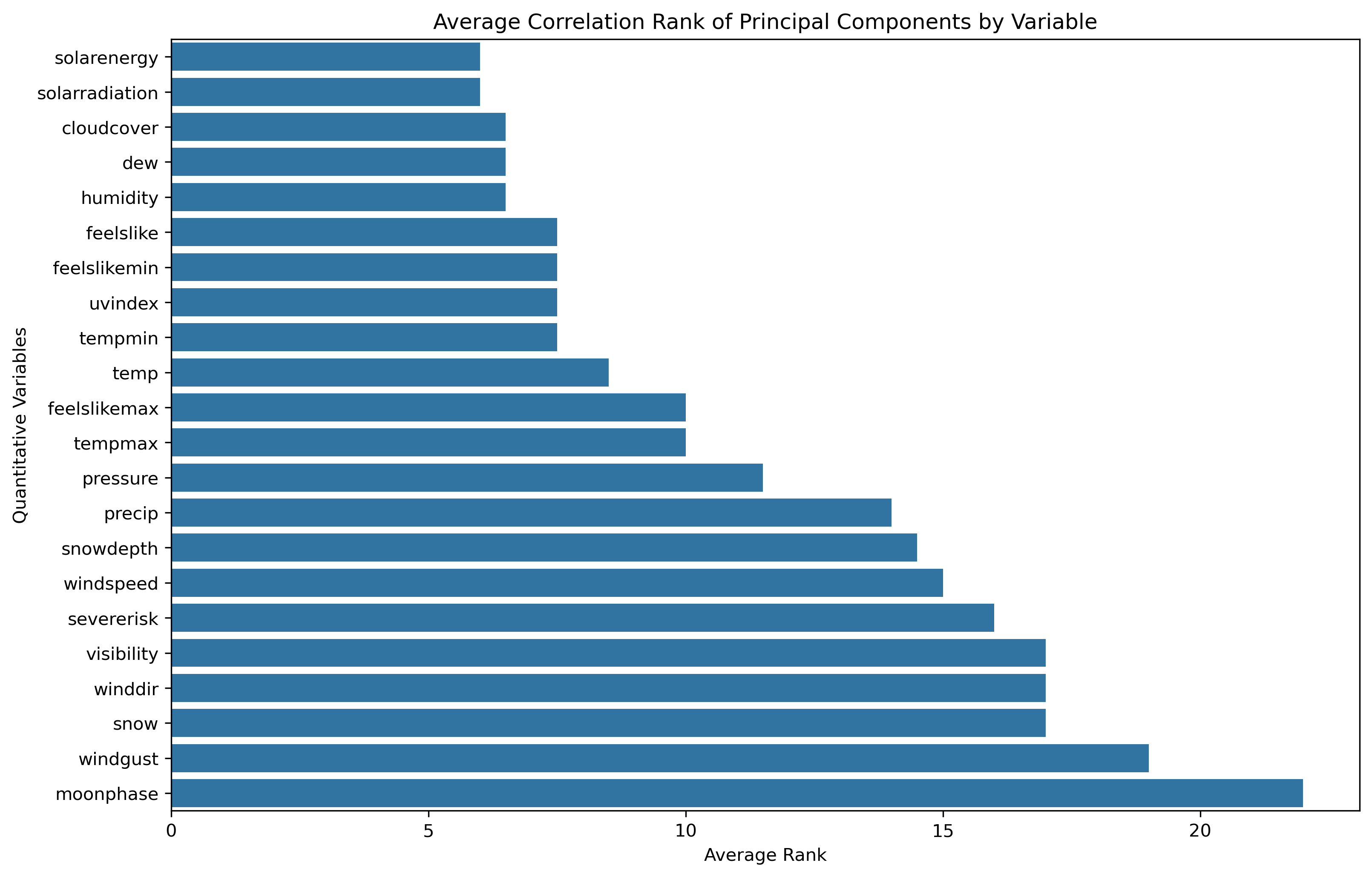
Loadings - Boxplot
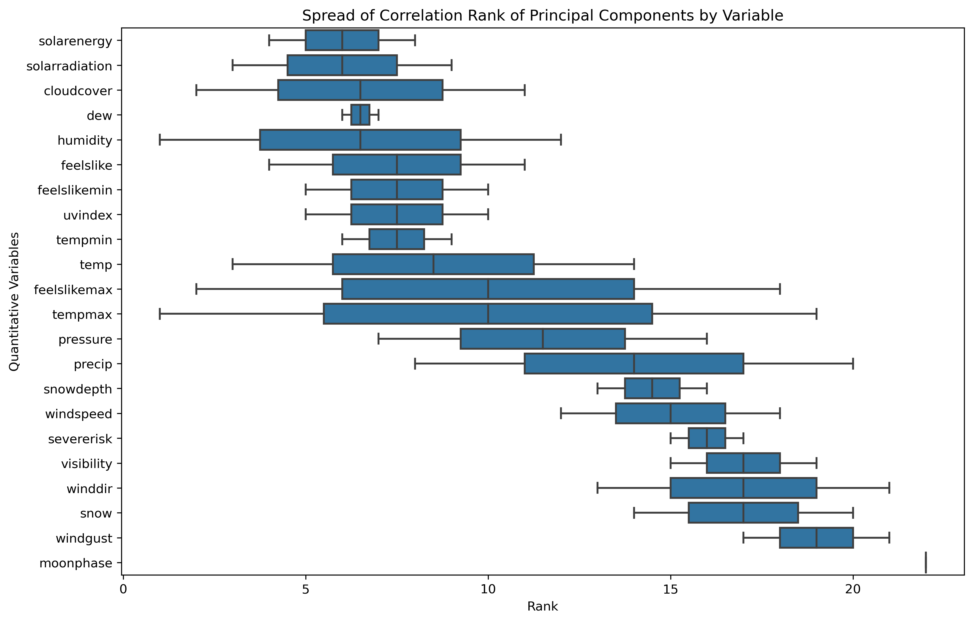
Again, the loadings matrix for two dimensional PCA shows different influence across the original data features. Moonphase is close to not having any influence on the two dimensional principal components.
Visualizing PCA in 2 Dimensions with Labels
The label of Weather Type was applied to the data projected onto the PCA space. This time, the data in its entirety was used.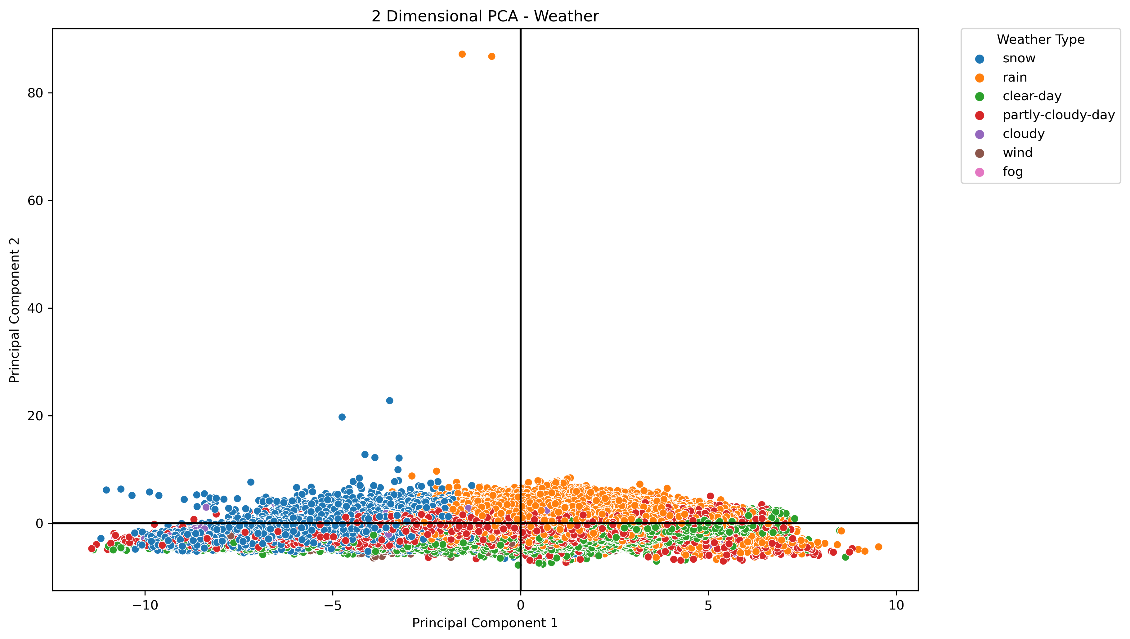
Explained and Cumulative Variance - Table
| principal_components | explained_variance | cumulative_variance |
|---|---|---|
| principal_component_1 | 33.12% | 33.12% |
| principal_component_2 | 28.13% | 61.25% |
Explained and Cumulative Variance - Visual
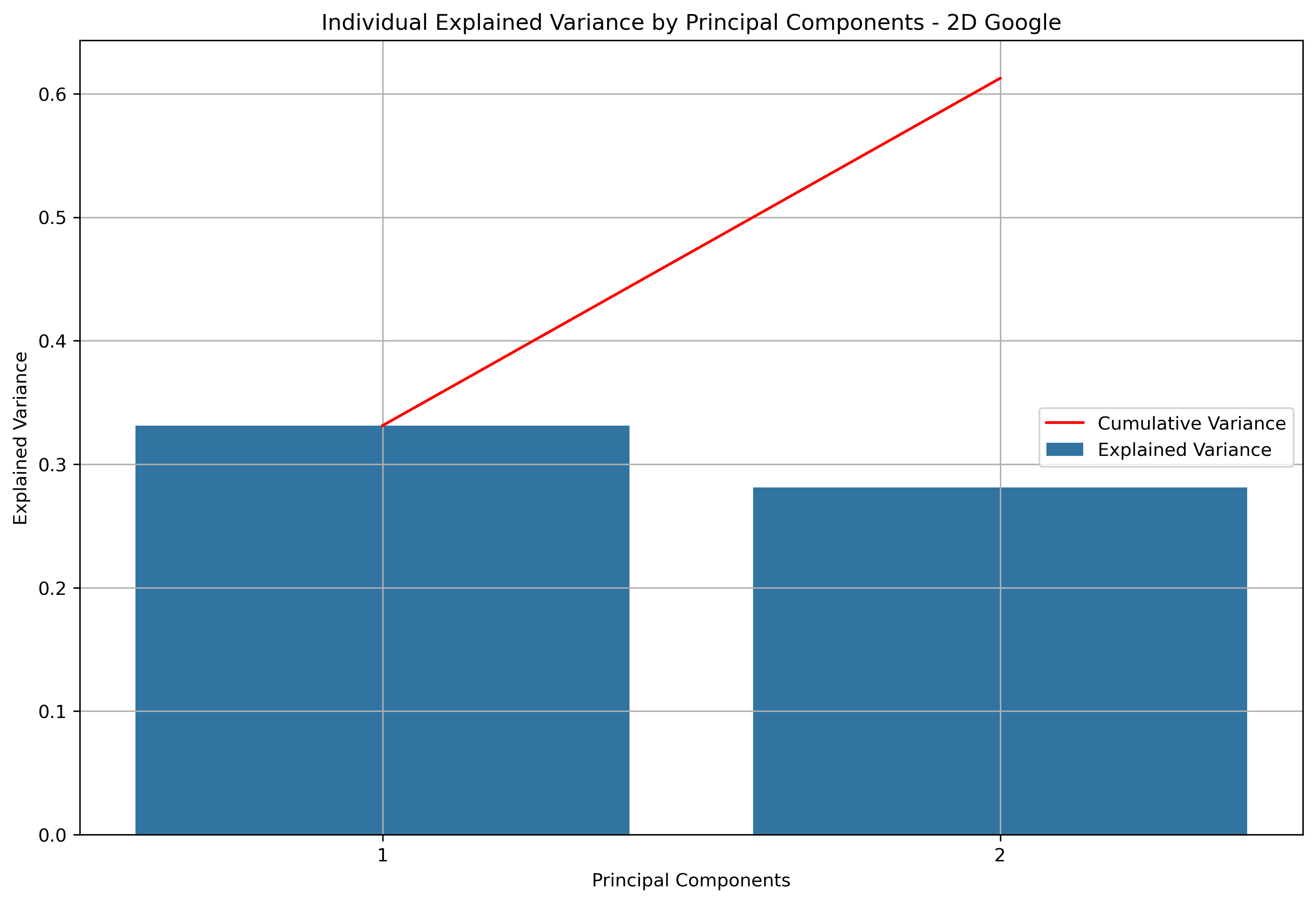
For two dimensional principal component analysis, 61.25% of information is retained from the original data.
Loadings - Table
| Feature | principal_component_1 | principal_component_2 |
|---|---|---|
| Latitude | 0.704954 | 0.054736 |
| Longitude | -0.693377 | -0.133590 |
| rating | -0.046771 | 0.706612 |
| total_ratings | -0.141710 | 0.692717 |
Loadings - Barplot

Loadings - Boxplot
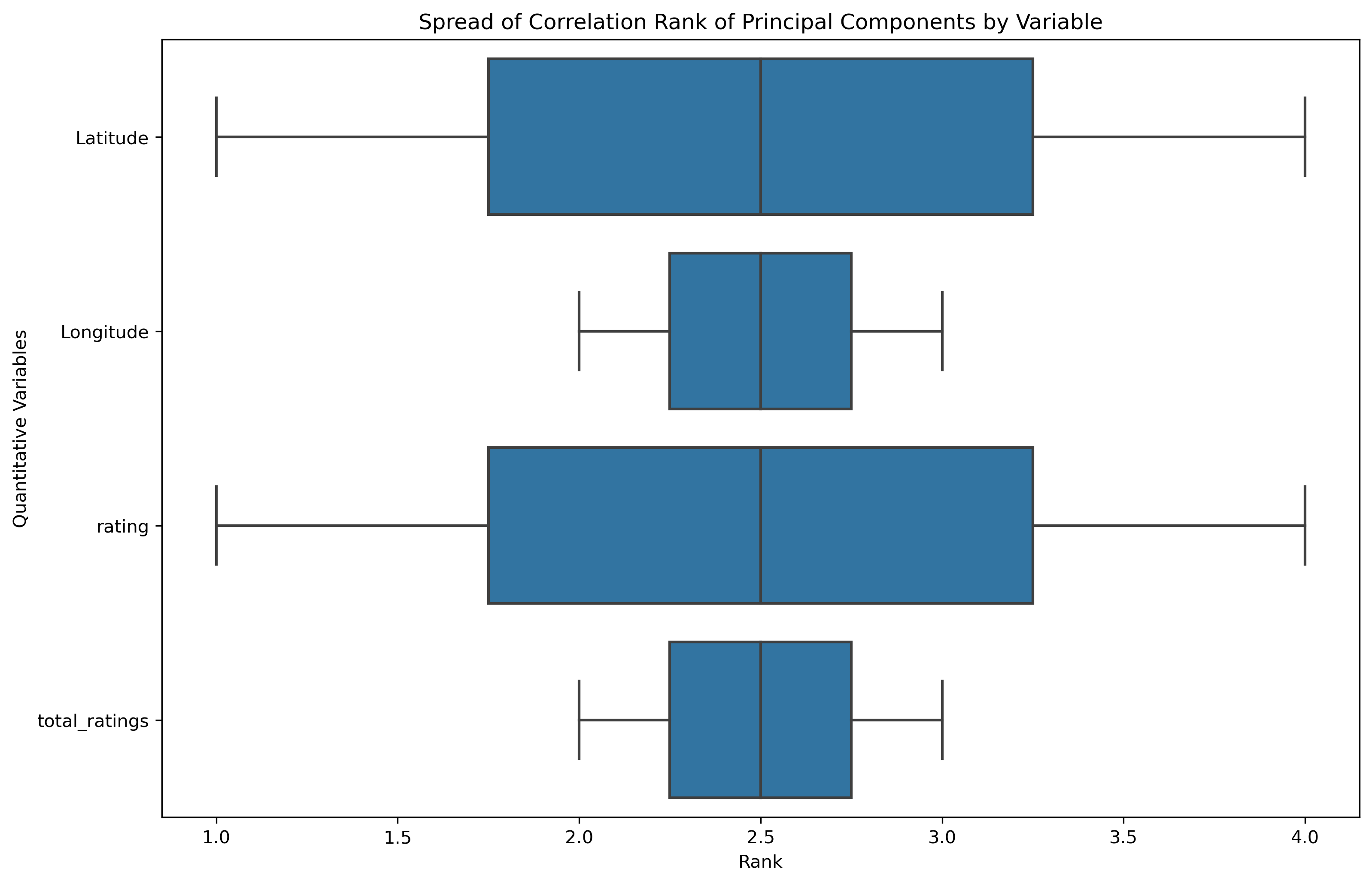
There is a slight difference between the loadings matrix in two dimensional PCA compared to the full dimensional PCA.
Visualizing PCA in 2 Dimensions with Labels
The label of business category was applied to the data projected onto the PCA space. This time, the data in its entirety was used, and an interesting pattern was created.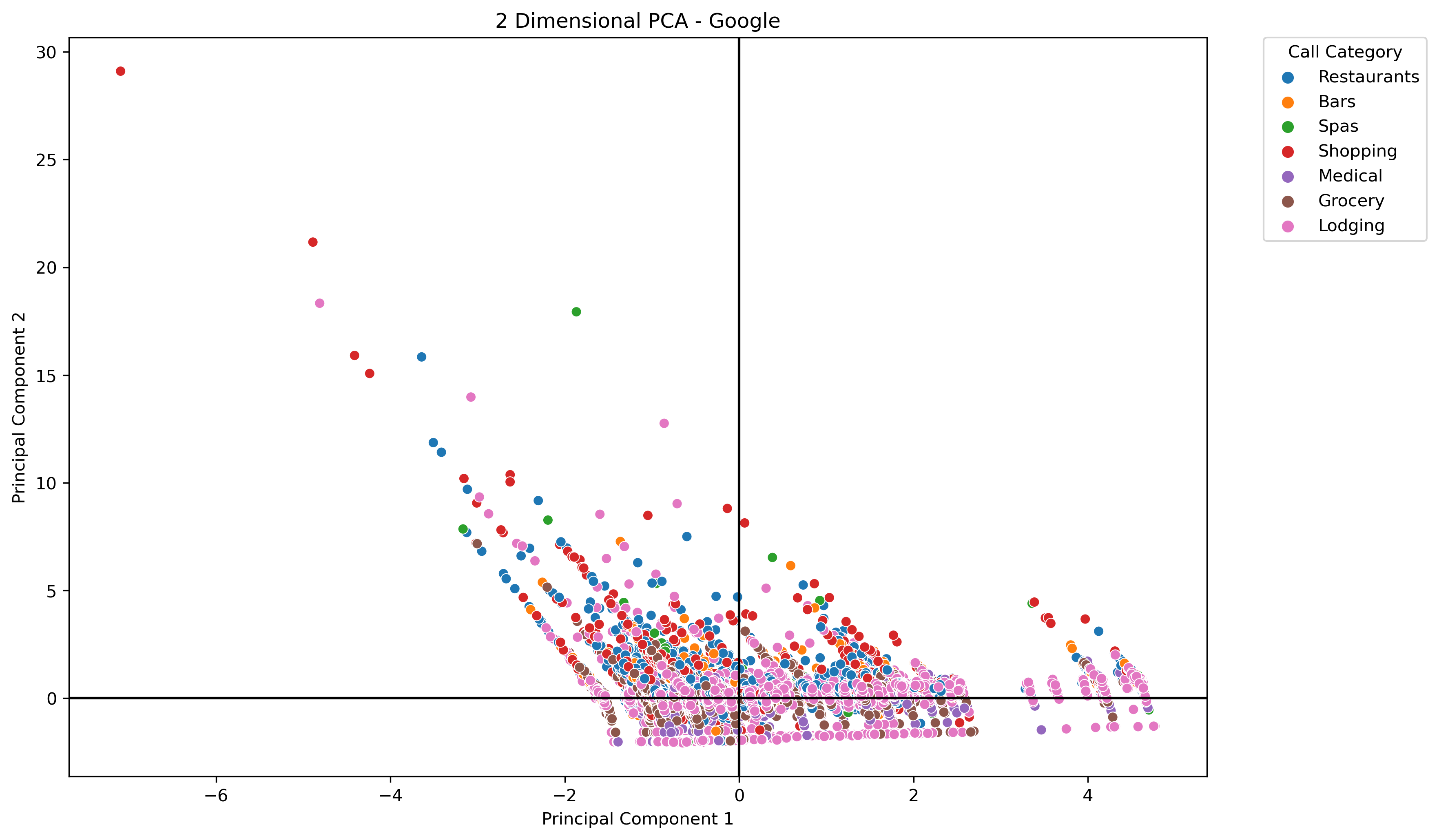
Summary of PCA Results and Analysis
Principal Component Analysis was applied to three main datasets relevant to this topic. Full Feature PCA, Three Dimensional PCA, and
Two Dimensional PCA results were analyzed. Specifically, eigenvectors and eigenvalues from the data projected into PCA spaces were investigated, with emphasis on how much information was retained by the
PCA process. An additional component of the analysis used loadings matrices in an attempt to understand the strength and direction each original feature had on the principal componets (new features).
Illustrations of the projected data were made for three dimensionsal PCA and two dimensional PCA, with labels applied to help detect potential patterns.
Some interesting takeaways:
- Loadings matrices and subsequently the influence of the original features on the principal components changed with reduced principal components, namely in the datasets with a greater number of features.
- Visualizations on the resort data with different labels did reveal some relevant cluster patterns.
- Visualizations on the weather data also revealed some relevant cluster patterns, and was the most symmetric of the three datasets when projected into the PCA space.
- Visualizations on the google places data did have some relevant cluster patterns revealed, but the data projected into the PCA space produced an overall shape much different to the other datasets. Even though outliers were addressed while cleaning this data, could hidden outliers be responsible for the uniqueness of the PCA projection results?