Modeling - Support Vector Machines
Overview of SVM
Support Vector Machines (SVMs) are supervised learning methods which transform features into a higher dimensional space to separate the labels. The usefulness of an SVM comes from when the input data in its original dimensional space isn’t linearly separable, but in a higher dimensional space there exists a hyperplane which can linearly separate the groups of the data.
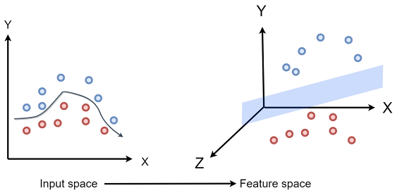
In the example above, the groups in the data are not linearly separable in their original two-dimensional space, however, transformed into a three-dimensional space, a three-dimensional plane is able to linearly separate the data. A hyperplane which exists in 4 or more dimensions, although it cannot be visualized, can be conceptualized mathematically and theoretically.
SVMs use a quadratic optimization algorithm, in which the final optimal dual form contains a dot product (or inner product). This allows for the use of kernels, which are functions that return an inner product in a higher dimensional space. Being able to apply kernels is essential, as just the solution to the dot product is needed and doesn’t actually need to be transformed into a higher dimensional space in practice. The example above takes a small amount of data in 2-dimensions and transforms them into 3-dimensions. However, if millions of points of data are transformed into a dimensional space in the thousands (or even into an infinite dimensional space), the problem becomes intractable. To reiterate, being able to use a dot product, and subsequently a kernel, allows for just the solution of the dot product to be used instead of actually transforming the data into a higher dimensional space. This makes SVMs highly efficient. Additionally, SVMs create a margin between the groups in the higher dimensional space. Any point on the margin is known as a support vector. Not only are they computationally efficient but they are also more resistant to outliers and noise due to this. Keep in mind that a single SVM is a binary classifier, however multiple SVMs can be ensembled together for more than a 2-class problem
Ommitting the initial mathematics to obtain the final optimal dual form, the main equation becomes:
In otherwords, solve for:
With the following constraints:
\[\text{Minimize } w, b \]
Maximizing and Minimizing these constraints now becomes an optimization problem:
\[\frac{\partial L}{ \partial b} = -\sum_{i} \lambda_i y_i = 0 \rightarrow \sum_{i} \lambda_i y_i = 0 \]
\[\frac{\partial L}{ \partial \lambda} = \sum_{i} y_i w^T \cdot x_i + b - 1 = 0 \rightarrow \sum_{i} y_i w^T \cdot x_i + b - 1 = 0 \]
Finally, substituting these optimal results into L gives:
\[\text{With } y_i(w^T x_i + b) - 1 = 0 \]
Where:
- The \( y_i \)'s are the label or group of data (usually represented by \( +1 \) and \( -1 \))
- The \( \lambda_i \)'s are the Lagrange Multipliers
- The \( x_i \)'s are the data vectors, and \( x_i^T x_j \) is the dot product
- The \( \lambda_i \)'s and \( y_i \)'s are scalars, while the \( x_i \)'s are vectors of data in their original dimensional space
There are several common kernels used with the SVM technique.
Essentially, if a potential fucntion for SVM can be written as an inner product, then it can be used as a kernel in SVM.
This section will talk about the Polynomial Kernel and the Radial Basis Function (RBF) Kernel.
- Polynomial Kernel
- Function: \( (a^Tb + r)^d \)
- \( a \text{ and } b \) are vectors
- \( r \) is the coefficient of the polynomial, which helps to control the size of the margin
- \( d \) is the degree of the polynomial, which helps control the comlexity of the model
- Idea: Uses a polynomial function to map the data into a higher-dimensional space by taking the dot product of the data in the original dimensional space and mapping this to the higher dimensional space with the polynomial function
- RBF Kernel
- Function: \( e^{-\gamma (a - b)^2} \)
- \( a \text{ and } b \) are vectors
- \( \gamma \) scales the result, and represents \( \frac{1}{2 \sigma^2} \)
- By substituting \( \gamma \) back in, the normal distribution formula is created, thus the RBF is based on the normal distribution
- Idea: Using the Gaussian function, the RBF kernel maps the data into an infinite-dimensional space
- Even a function which maps data into an infinite space can be shown to be a kernel (i.e. written as a dot product)
Simple Example With the Polynomial Kernel
Given a Polynomial Kernel with parameters \( r = 1, d = 2 \) on data in an original 2-dimensional dataset:
This can be shown to a be a dot product which can "cast" points into the proper number of dimensions:
\[= (a^Tb)^2 + 2a^Tb + 1 \]
\[\text{Given 2D Vectors: } a = [a_1, a_2], b = [b_1, b_2] \rightarrow \]
\[(a^Tb)^2 + 2a^Tb + 1 = (a_1b_1 + a_2b_2)^2 + 2(a_1b_1 + a_2b_2) + 1 \]
\[= a_1^2b_1^2 + 2a_1b_1a_2b_2 +a_2^2b_2^2 + 2a_1b_1 + 2a_2b_2 + 1 \]
\[= a_1^2b_1^2 + 2a_1b_1a_2b_2 +a_2^2b_2^2 + 2a_1b_1 + 2a_2b_2 + 1 \]
This can be written as a dot product of two transformed points, \( transform_{1} \cdot transform_{2} \):
\[transform_{1} \cdot transform_{2} = a_1^2b_1^2 + 2a_1b_1a_2b_2 +a_2^2b_2^2 + 2a_1b_1 + 2a_2b_2 + 1 \]
\[transform_{1} = [a_1^2, \sqrt{2} a_1a_2, a_2^2, \sqrt{2} a_1, \sqrt{2} a_2, 1] \]
\[transform_{2} = [b_1^2, \sqrt{2} b_1b_2, b_2^2, \sqrt{2} b_1, \sqrt{2} b_2, 1] \]
Thus, 2-dimensional data is "cast" or "projected" into a 6-dimensional space.
Applying this to an example,
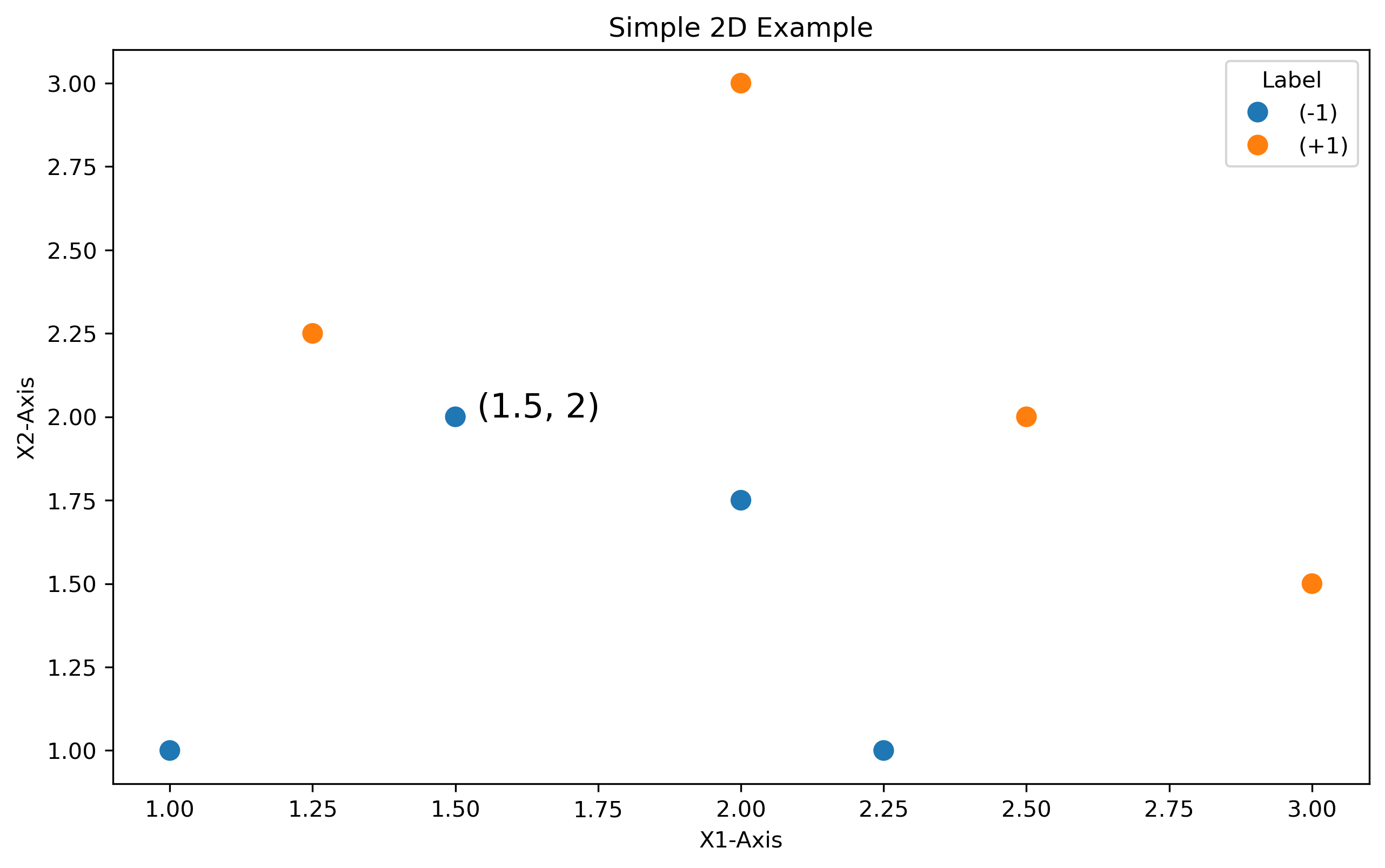
Finally, using a point from this data, \( a = [a_1, a_2] = [1.5, 2] \):
\[transform_{1} = [a_1^2, \sqrt{2} a_1a_2, a_2^2, \sqrt{2} a_1, \sqrt{2} a_2, 1] \]
\[ = [\frac{3}{2}^2, \sqrt{2} \frac{3}{2} 2, 2^2, \sqrt{2} \frac{3}{2}, \sqrt{2} 2, 1] \]
\[ = [\frac{9}{4}, 3 \sqrt{2}, 4, \frac{3}{2} \sqrt{2}, 2 \sqrt{2}, 1] \]
\[ \rightarrow \]
\[ = [1.5, 2] \rightarrow [\frac{9}{4}, 3 \sqrt{2}, 4, \frac{3}{2} \sqrt{2}, 2 \sqrt{2}, 1] \]
Data Preparation
To preface the data used in this, SVMs can only work on labeled numeric data. First, an SVM is a supervised machine learning method.
This means, that it can only be used on labeled data in order to train the model. Second, due to the mathematic nature of dot products, and
subsequently kernels, the data must be numeric.
The data used for this model will be the weather data featured in many of the models throughout this project. The goal will be to determine the
icon used by a weather system on a given day of data. Options will be:
- Clear Day
- Rain
- Snow
- Other
Note that SVMs are binary classifiers. When a multi-class problem is presented, ensemble learning must be used to link several SVM models together. However, libraries like Scikit-Learn automatically ensemble.
Certain numeric variables directly associated with Rain, Snow, and Wind were disregarded as these are essentially what is trying to be predicted in the categorical label of icon. The variables used in the analysis were:
- Maximum Temperature
- Minimum Temperature
- Temperature
- Fells Like Maximum (temperature)
- Fells Like Minimum (temperature)
- Feels Like (temperature)
- Dew Point
- Humidity
- Pressure
- Day of the Year
Using these numeric variables, principal component analysis (PCA) was performed to reduce the dimensionality of the data while retaining as much information as possible.
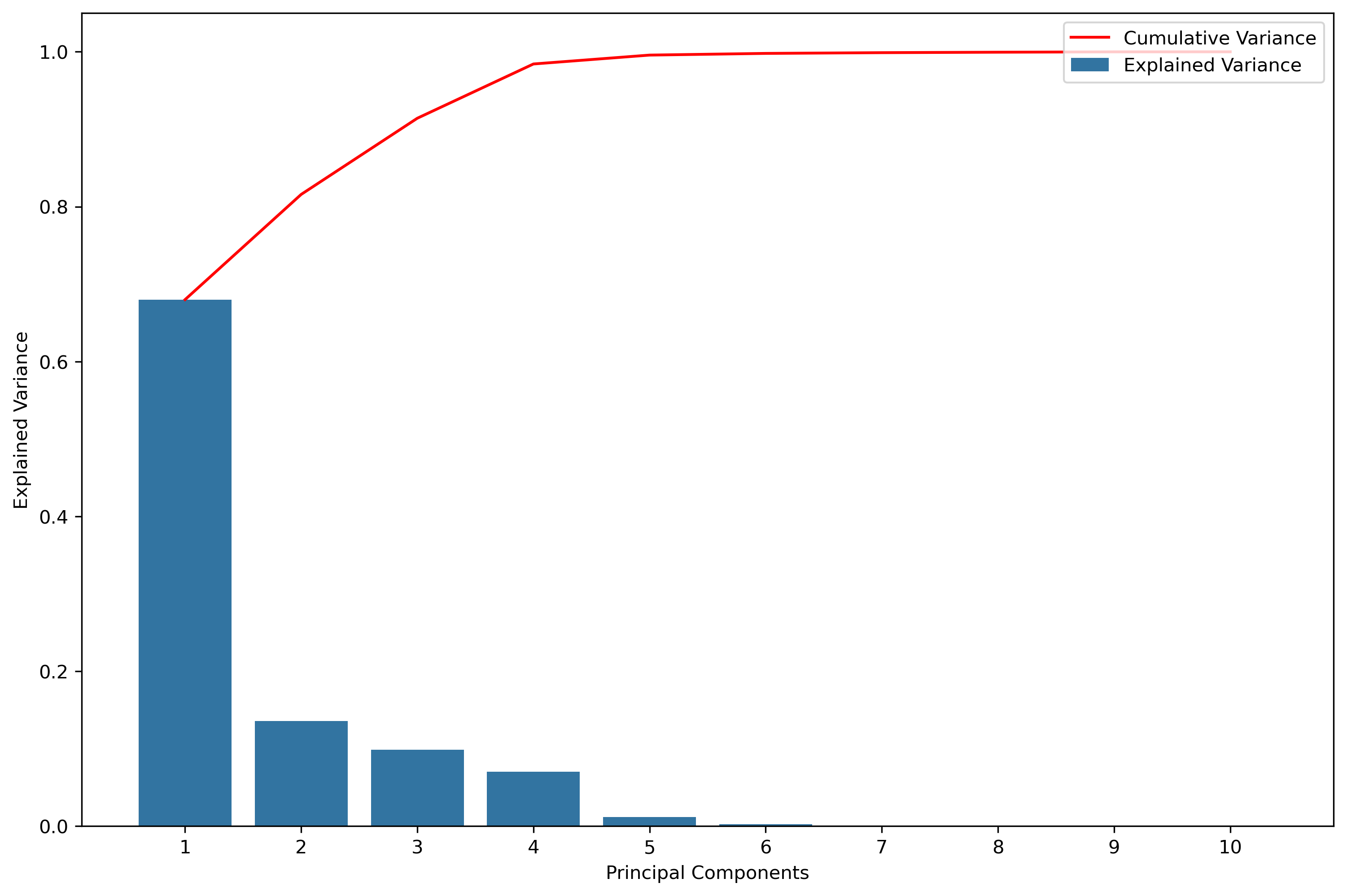
Utilizing PCA retains over 80% of information in the first two principal components, while over 90% is retained within the first three principal components. With over 80% of information retained with the first two principal components, these will be the data columns used. The upside to this is that the data will be known to begin in two-dimensions and trasnformed further.
Additionally, training and testing sets were created. The two sets are disjoint, and must be disjoint. Using non-disjoint data between testing and training won't give an accurate representation of the performance of the model. First, this could result in an overfit of the model, which could end up describing noise, rather than the underlying distribution. Second, the testing set being non-disjoint helps to represent real-world data (i.e. unseen data).
The explained processes above can be examined in the datasets below.
Weather Data
| datetime | tempmax | tempmin | temp | feelslikemax | feelslikemin | feelslike | dew | humidity | precip | precipprob | precipcover | snow | snowdepth | windgust | windspeed | winddir | pressure | cloudcover | visibility | solarradiation | solarenergy | uvindex | sunrise | sunset | moonphase | icon | stations | resort | tzoffset | severerisk | type_freezingrain | type_ice | type_none | type_rain | type_snow |
|---|---|---|---|---|---|---|---|---|---|---|---|---|---|---|---|---|---|---|---|---|---|---|---|---|---|---|---|---|---|---|---|---|---|---|---|
| 2019-01-01 | 16.4 | 2.0 | 7.0 | 10.2 | -13.3 | -0.6 | -1.2 | 69.1 | 0.008 | 100.0 | 20.83 | 0.0 | 20.7 | 18.30000 | 10.6 | 4.9 | 1014.5 | 59.0 | 8.6 | 116.8 | 9.9 | 5.0 | 07:26:20 | 16:51:51 | 0.85 | snow | ['72467523063', '72206103038', 'CACMC', 'KCCU', 'KEGE', 'KLXV', 'DJTC2', 'K20V', '72467393009'] | Vail | 0.0 | 0.0 | 0 | 0 | 0 | 0 | 1 |
| 2019-01-02 | 24.3 | -0.9 | 11.4 | 21.9 | -11.9 | 5.4 | -10.5 | 39.9 | 0.004 | 100.0 | 4.17 | 0.0 | 20.8 | 29.77377 | 8.7 | 353.1 | 1021.4 | 0.0 | 9.9 | 121.6 | 10.7 | 5.0 | 07:26:27 | 16:52:41 | 0.89 | snow | ['72467523063', '72206103038', 'CACMC', 'KCCU', 'KEGE', 'KLXV', 'DJTC2', 'K20V', '72467393009'] | Vail | 0.0 | 0.0 | 0 | 0 | 0 | 0 | 1 |
| 2019-01-03 | 29.0 | 5.3 | 17.6 | 21.9 | -4.0 | 8.6 | 4.1 | 56.1 | 0.004 | 100.0 | 4.17 | 0.2 | 20.8 | 32.20000 | 9.8 | 328.9 | 1024.7 | 0.0 | 9.8 | 123.3 | 10.6 | 5.0 | 07:26:31 | 16:53:33 | 0.92 | snow | ['72467523063', '72206103038', 'CACMC', 'KCCU', 'KEGE', 'KLXV', 'DJTC2', 'K20V', '72467393009'] | Vail | 0.0 | 0.0 | 0 | 0 | 0 | 1 | 1 |
| 2019-01-04 | 34.0 | 11.9 | 23.4 | 28.7 | 3.4 | 17.1 | 7.0 | 50.4 | 0.001 | 100.0 | 4.17 | 0.1 | 20.8 | 20.80000 | 9.0 | 311.0 | 1025.5 | 0.0 | 9.9 | 123.7 | 10.7 | 5.0 | 07:26:34 | 16:54:26 | 0.96 | snow | ['72467523063', '72206103038', 'CACMC', 'KCCU', 'KEGE', 'KLXV', 'DJTC2', 'K20V', '72467393009'] | Vail | 0.0 | 0.0 | 0 | 0 | 0 | 1 | 1 |
| 2019-01-05 | 34.1 | 14.3 | 27.1 | 29.4 | 4.3 | 20.1 | 1.9 | 33.9 | 0.001 | 100.0 | 4.17 | 0.0 | 20.4 | 20.80000 | 10.1 | 243.5 | 1022.2 | 19.4 | 9.7 | 110.3 | 9.6 | 5.0 | 07:26:34 | 16:55:20 | 0.00 | rain | ['72467523063', '72206103038', 'CACMC', 'DYGC2', 'KCCU', 'KEGE', 'KLXV', 'DJTC2', 'K20V', '72467393009'] | Vail | 0.0 | 0.0 | 0 | 0 | 0 | 1 | 1 |
| 2019-01-06 | 29.9 | 18.5 | 25.9 | 22.4 | 5.1 | 16.1 | 18.1 | 72.5 | 0.035 | 100.0 | 58.33 | 0.6 | 20.6 | 33.30000 | 16.9 | 266.7 | 1009.3 | 78.7 | 6.3 | 47.3 | 4.1 | 2.0 | 07:26:32 | 16:56:16 | 0.02 | snow | ['72467523063', '72206103038', 'CACMC', '72038500419', 'DYGC2', 'KCCU', 'KEGE', 'A0000594076', 'KLXV', 'DJTC2', 'K20V', '72467393009'] | Vail | 0.0 | 0.0 | 0 | 0 | 0 | 1 | 1 |
| 2019-01-07 | 24.8 | 14.7 | 20.3 | 12.8 | 2.5 | 6.5 | 13.7 | 75.2 | 0.004 | 100.0 | 8.33 | 0.4 | 21.3 | 45.70000 | 27.9 | 271.2 | 1015.6 | 83.7 | 4.8 | 35.8 | 3.0 | 2.0 | 07:26:27 | 16:57:13 | 0.06 | snow | ['72467523063', '72206103038', 'CACMC', 'DYGC2', 'KCCU', 'KEGE', 'KLXV', 'DJTC2', 'K20V', '72467393009'] | Vail | 0.0 | 0.0 | 0 | 0 | 0 | 0 | 1 |
| 2019-01-08 | 34.6 | 17.2 | 25.1 | 34.6 | 5.0 | 17.8 | 12.0 | 59.5 | 0.013 | 100.0 | 8.33 | 0.0 | 21.3 | 27.70000 | 15.2 | 312.1 | 1029.4 | 34.5 | 9.5 | 122.9 | 10.5 | 5.0 | 07:26:21 | 16:58:11 | 0.09 | rain | ['72467523063', '72206103038', 'CACMC', 'KCCU', 'KEGE', 'KLXV', 'DJTC2', 'K20V', '72467393009'] | Vail | 0.0 | 0.0 | 0 | 0 | 0 | 1 | 1 |
| 2019-01-09 | 38.3 | 23.0 | 28.6 | 38.3 | 13.6 | 22.6 | 9.9 | 45.4 | 0.000 | 0.0 | 0.00 | 0.0 | 21.2 | 23.00000 | 13.0 | 142.9 | 1029.6 | 1.0 | 9.9 | 114.0 | 9.8 | 5.0 | 07:26:12 | 16:59:11 | 0.12 | clear-day | ['72467523063', '72206103038', 'CACMC', 'KCCU', 'KEGE', 'KLXV', 'DJTC2', 'K20V', '72467393009'] | Vail | 0.0 | 0.0 | 0 | 0 | 1 | 0 | 0 |
| 2019-01-10 | 33.7 | 17.0 | 26.4 | 33.7 | 9.8 | 22.6 | 14.3 | 60.6 | 0.026 | 100.0 | 12.50 | 0.8 | 21.4 | 17.20000 | 8.8 | 323.7 | 1023.3 | 39.9 | 8.3 | 75.9 | 6.6 | 4.0 | 07:26:01 | 17:00:11 | 0.16 | snow | ['72467523063', '72206103038', 'CACMC', 'KCCU', 'KEGE', 'KLXV', 'DJTC2', 'K20V', '72467393009'] | Vail | 0.0 | 0.0 | 0 | 0 | 0 | 1 | 1 |
Data Prepared for SVM
| principal_component_1 | principal_component_2 | principal_component_3 | icon |
|---|---|---|---|
| 0.942514 | -0.576079 | 1.198957 | clear-day |
| 2.654999 | -1.275326 | -0.361316 | clear-day |
| -3.673853 | -0.740941 | -0.592327 | clear-day |
| -2.647318 | -0.719348 | -0.666917 | clear-day |
| 1.727955 | -2.687412 | -2.064494 | clear-day |
| 2.084569 | -3.050954 | 0.370595 | clear-day |
| 0.332007 | -1.827508 | -0.512350 | clear-day |
| 2.675351 | -2.042598 | -1.612940 | clear-day |
| 2.586008 | -0.613561 | -0.373239 | clear-day |
| 4.194451 | -0.092180 | -0.290021 | clear-day |
Training Data for SVM
| principal_component_1 | principal_component_2 | principal_component_3 | icon |
|---|---|---|---|
| -1.002711 | 0.631963 | 1.020450 | rain |
| 1.810245 | 0.472562 | -0.984442 | rain |
| -1.321761 | 0.328007 | -1.294977 | snow |
| -2.113220 | -2.441253 | 2.112451 | clear-day |
| -2.825162 | 0.377729 | -1.194965 | other |
| 2.831919 | -1.425390 | -0.509642 | clear-day |
| -1.233084 | -0.879615 | -0.410951 | clear-day |
| -6.344406 | -1.297544 | -0.659969 | snow |
| -1.140114 | -0.625937 | -1.057581 | other |
| -1.529002 | -0.796274 | 1.207417 | clear-day |
Testing Data for SVM
| principal_component_1 | principal_component_2 | principal_component_3 | icon |
|---|---|---|---|
| -2.238822 | -1.044349 | 1.775507 | clear-day |
| 2.225502 | -2.320712 | 0.050504 | clear-day |
| -0.527601 | -1.791034 | -0.212053 | clear-day |
| 3.215091 | 1.111794 | 0.390800 | rain |
| -3.210906 | -0.738177 | 2.299730 | clear-day |
| 2.082178 | -1.067775 | -0.344255 | clear-day |
| -0.087810 | -0.396630 | 1.701564 | other |
| -0.001700 | -1.168685 | 1.564984 | other |
| -2.811564 | 0.662677 | -0.811092 | snow |
| 0.477921 | -0.575362 | -0.571819 | clear-day |
Coding SVM
The code for the data preparation and performing SVM can be found [here].
The kernels mentioned in the overview, Polynomial and RBF will be used. Additionally, a third kernel known as the Sigmoid Kernel will be used as well. Different cost parameters will be utilized to
find the best model.
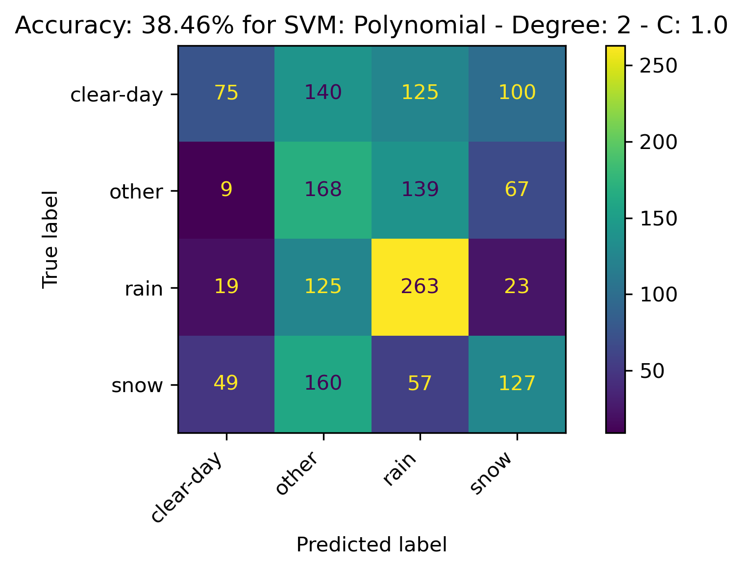
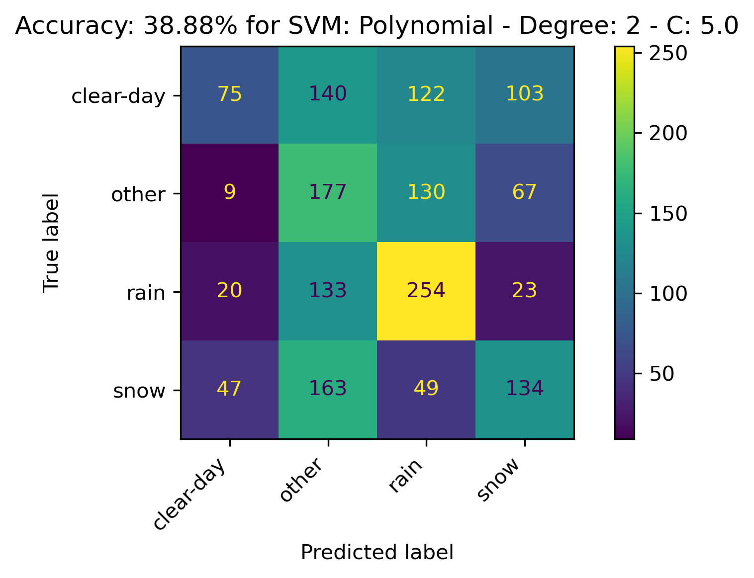
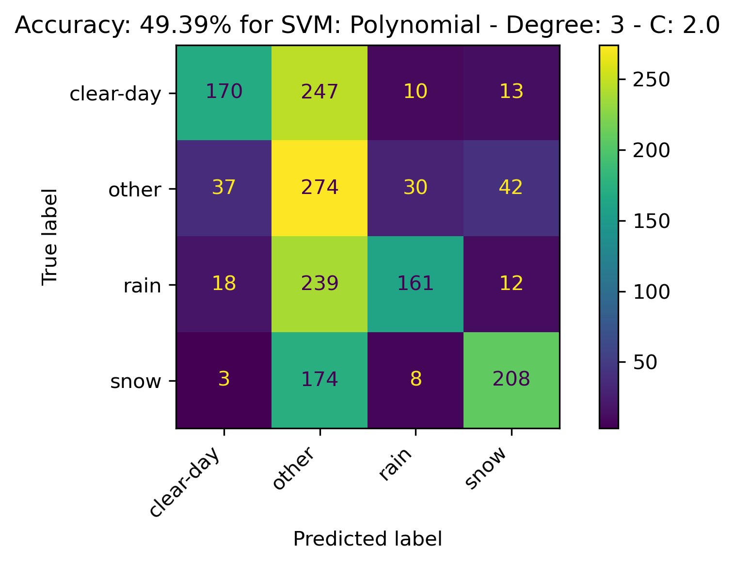
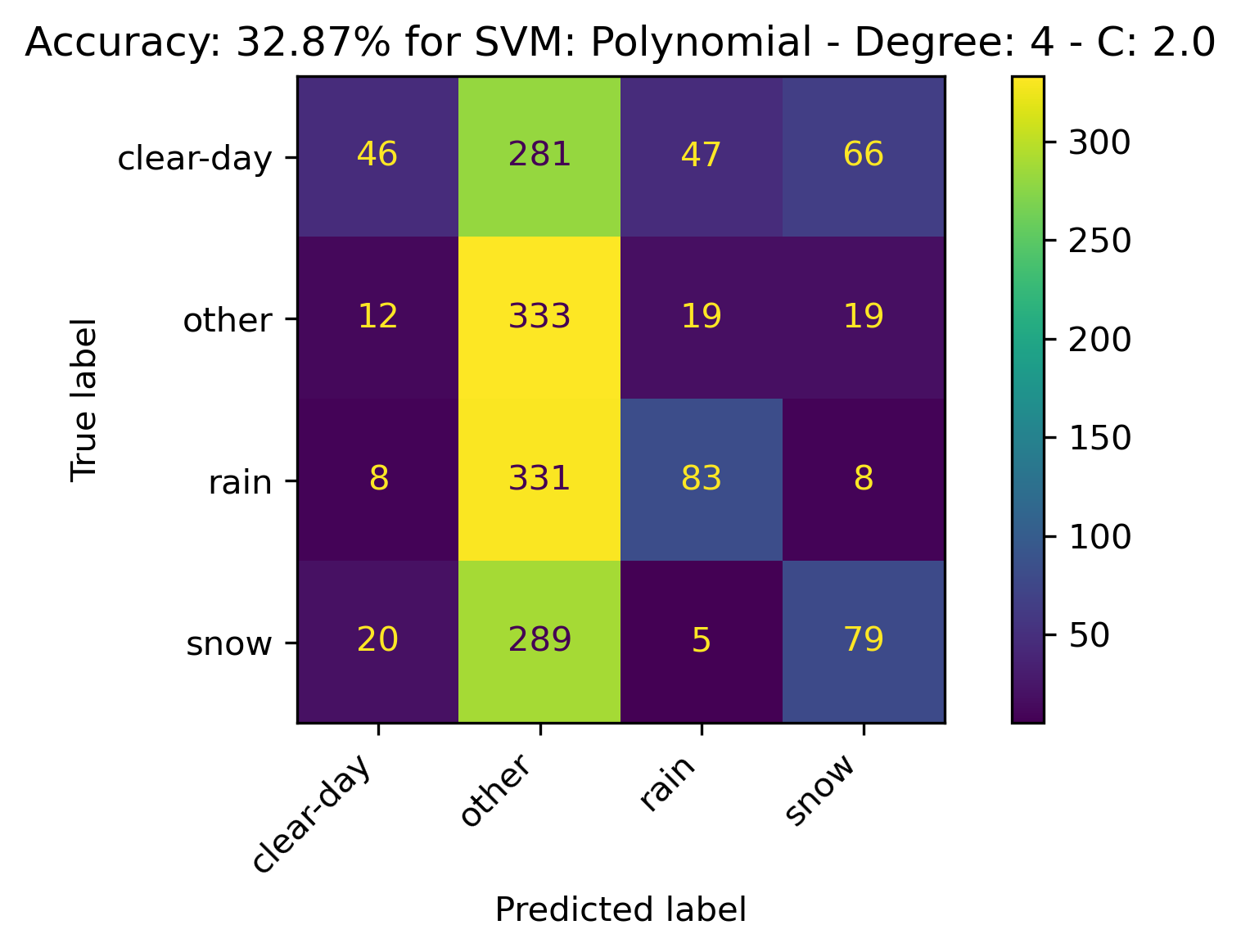
Polynomial Kernel
For the Polynomial Kernel, the kernel with the following parameters performed the best:
- Degree: 3
- C: 2.0
-
The confusion matrices and results are listed below.
RBF Kernel
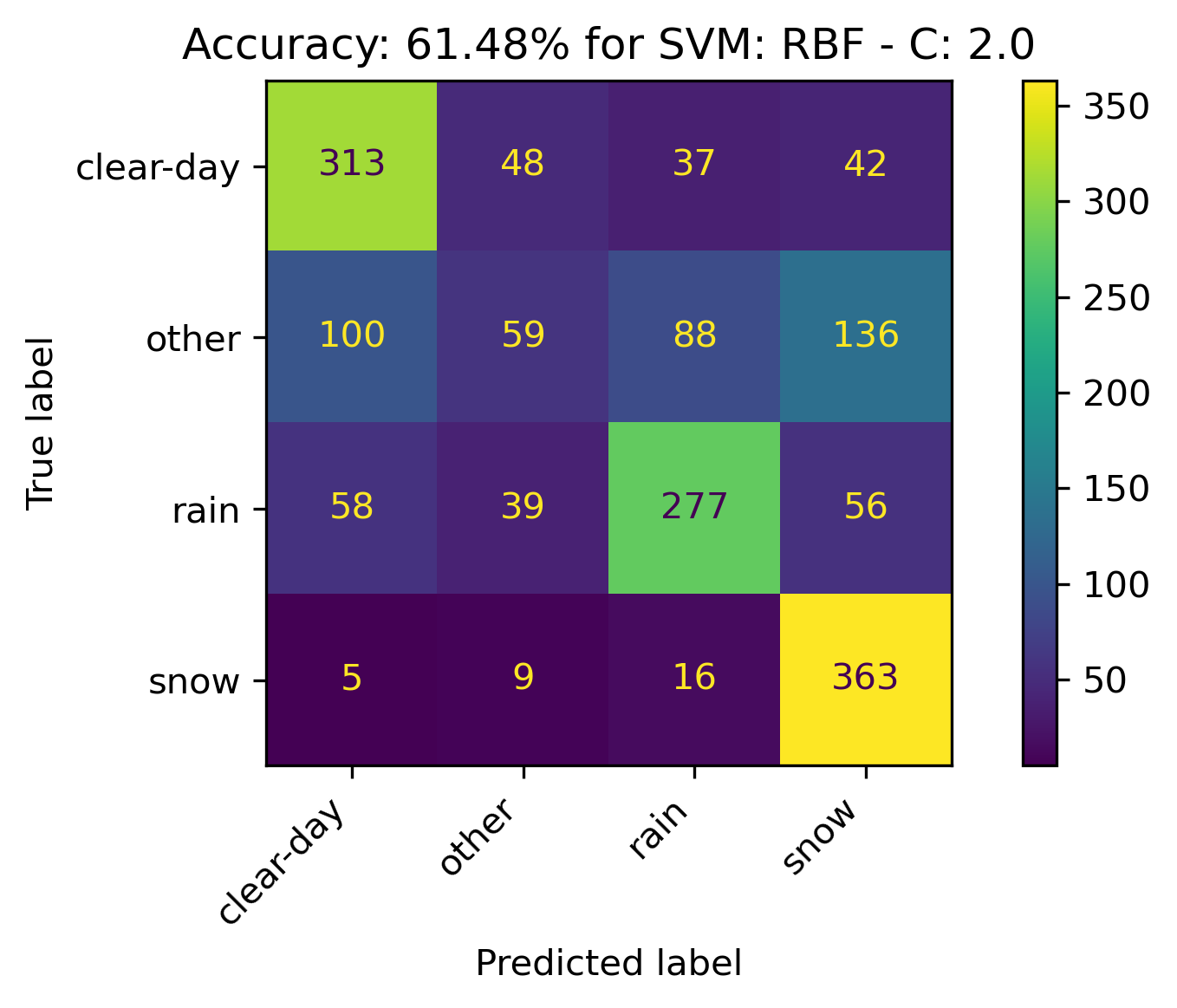
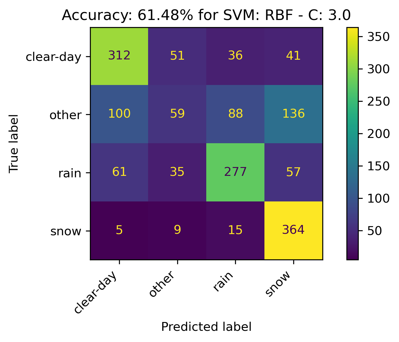
For the RBF, altering C only seemed to slightly change the confusion matrix while the overall accuracy remained the same. Therefore, it makes sense to leave the C value at the default of 1.
- C: 1.0
-
The confusion matrices and results are listed below.
Sigmoid Kernel
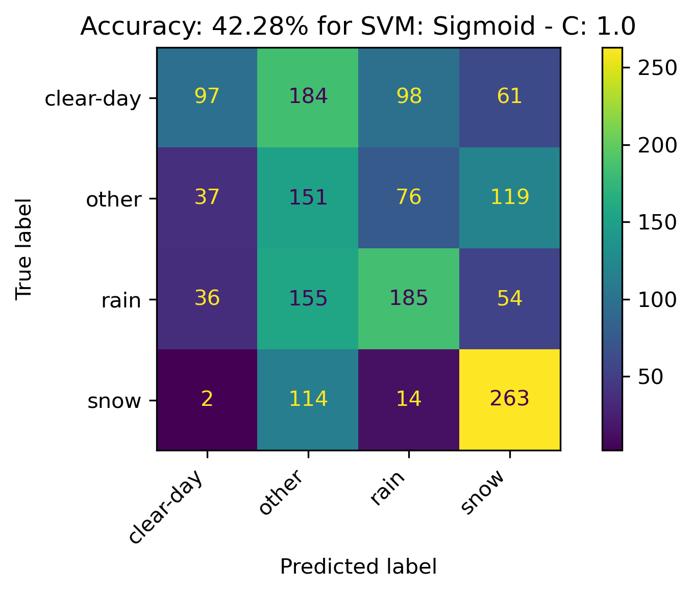
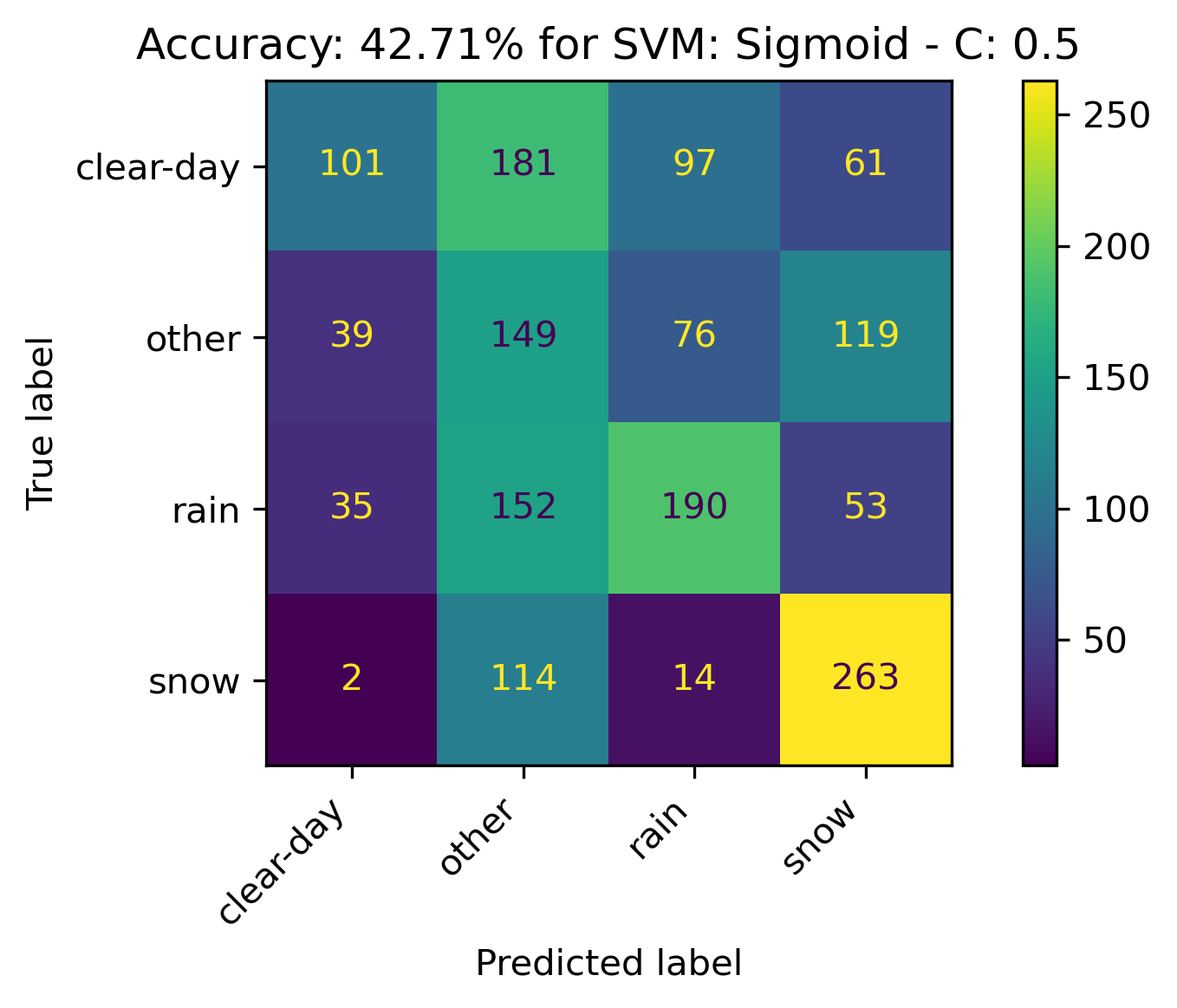
For the Sigmoid, increasing C seemed to decrease the accuracy. Thus a final C value was tested in the opposite direction to obtain optimal results.
- C: 0.5
-
The confusion matrices and results are listed below.
SVM Results
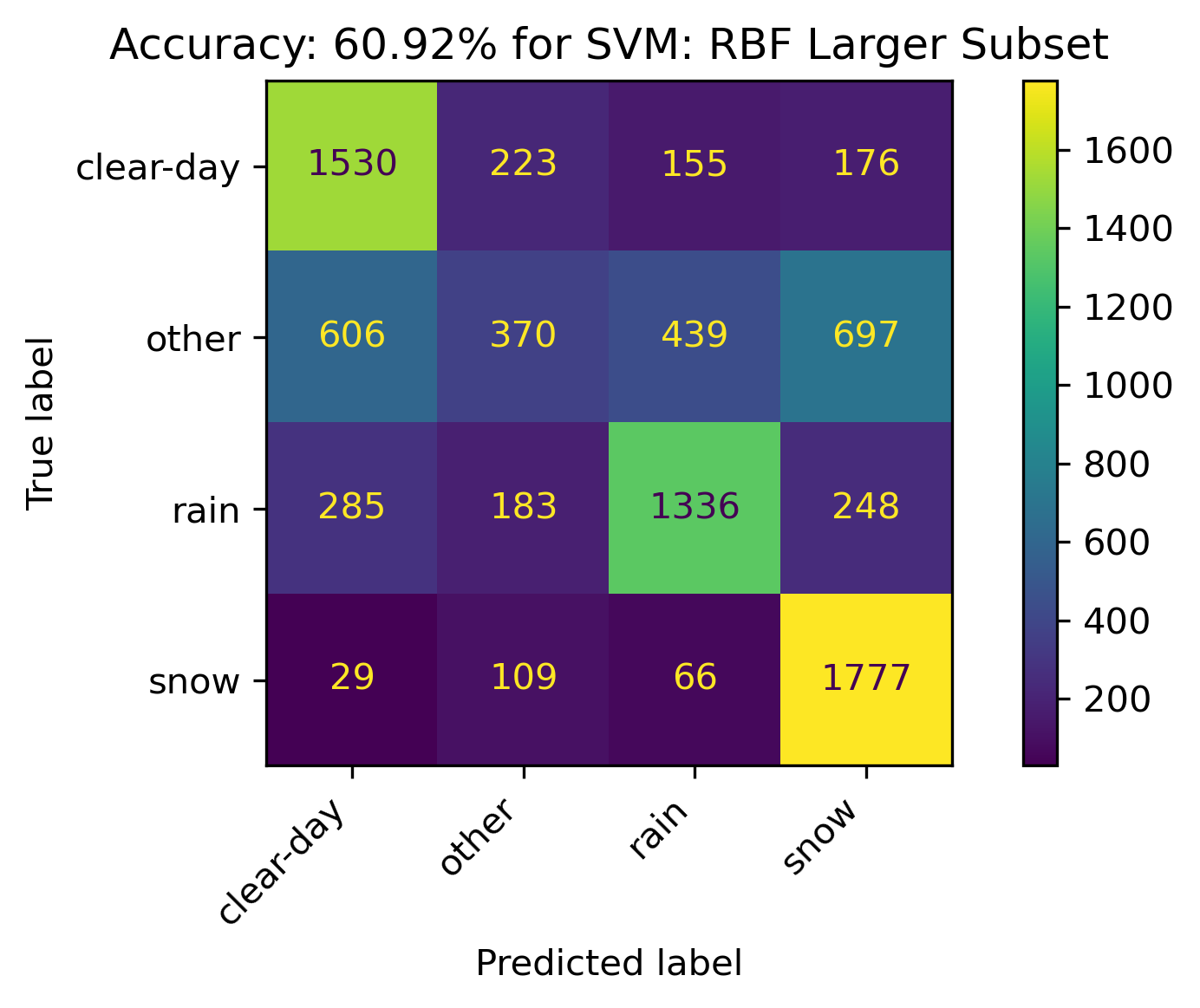
Although not extremely desirable results, the RBF with the default cost parameter of C = 1.0 performed the best overall. To
illustrate these results, a larger subset of 5% of the data on 3 principal components was trained. This resulted in an accuracy of 60.92%.
SVM Conclusions
An analysis was performed to examine if a better method to categorize the weather for a given day existed. The possible categories that could result were Clear, Rain, Snow, or Other. Overall, the categories of Clear, Rain, and Snow were able to be predicted with decent accuracy. However, the category of Other was more difficult to predict given the models provided. Interestingly enough, when predicting between Snow and Rain, there is a less of chance to falsely predict this. In other words, on days when it would snow or rain, if they were incorrectly predicted, out of the potential categories, it's more likely to be predicted as either Clear or Other. Other contains phenomena such as fog, wind, and overcast.
