Modeling - Regression
The Link Between Linear Regression and Logistic Regression
Define and explain linear regression.
Linear Regression is a parametric model which attempts to learn the best weights and biases to create a line to fit data, suited for quantitative data with a linear relationship. The weights and biases are the parameters. Normally, ordinary least squares is used to minimize the sum of squared errors. Ordinary least squares requires an algebraic solution between matrices of the data. This is a regression problem, so it is mostly used to predict continous values which could have an infinite range of values.
Define and explain logistic regression.
Logistic Regression is a parametric model which attempts to learn the best weights and biases to predict a value between 0 and 1, suited for binary categorical data. The weights and biases are the parameters. Normally, the model is trained by optimizing a log likelihood function. This optimization problem can sovled via different loss functions through gradient ascent (maximization) or gradient descent (minimization). The result from a Logistic Regression problem is a value between 0 and 1, and there is usually a threshold (standard of 0.5) to assign to one of the binary labels.
How are they similar and how are they different?
The history behind the creation of Logistic Regression is closely related to Linear Regression. A prediction of Linear Regression can roughly be represented in matrix format by the data, weights, and bias \(y=w^tx + b\). The result of the Linear Regression predictions exists in an infinite range \(y\in [-\infty, +\infty]\). Logistic Regression was created by applying a function \(H(x)\) to that linear equation to confine the results between 0 and 1, resulting in \(H(x)\in [0, 1]\).
Does logistic regression use the Sigmoid function?
The function that is applied to the equation with the linear relationship to bound the results between 0 and 1 is known as the Sigmoid Function. Given \(z=w^tx + b\), this is set equal to a log odds formula, known as the logit function, ( \(\log{\frac{p}{1-p}}=w^tx + b\) ), and solved for p to give \(p=\frac{1}{1+e^{-z}}\). This is known as the Sigmoid function, also called the logsitc function or inverse logit function. The Sigmoid function is bounded between 0 and 1, and then used to create a likelihood equation.
Explain how maximum likelihood is connected to logistic regression.
After the Sigmoid function is created, the goal becomes to learn the parameters (\(\theta\)), which are the weights and biases within the inital linear equation. This is accomplished by setting up a Bernoulli type equation between the probability being one of the binomial labels given the parameters. This Bernoulli type equation is then multiplied across all datapoints, setting up a likelihood problem. The goal of Logistic Regression is to maximize this likelihood problem, thus resulting in maximum likelihood. In fact, the logarithm of this is optimized, due to its monotonic properties.
Code
The script for this coding section can be found [here].
Data Preparation
The setup for this section uses the Ski Resort data. The goal for these models will be create a binary label problem with the attempt to predict country using characteristics of ski resorts. The countries in question are the United States and Canada (i.e. the label options). The actual data will be the following characteristics:
- Trails Easy: the number of easy trails at a ski resort
- Trails Intermediate: the number of medium trails at a ski resort
- Trails Difficult: the number of difficult trails at a ski resort
- Lifts: the number of lifts at a ski resort
The data is cleaned as is, however, some of the trails and lifts have decimals due to the ski resort statistical website reporting some trails and lifts as partial. To fix this, any partial characteristics were simply rounded to the nearest integer.
Logistic Regression itself is able to take diverse numerical data, however, this data also needs to be prepared for multinomial regression. With this in mind, the decision to use count type data was made.
Initial Data
The starting data for this analysis was the Ski Resort dataset. A snippet is below:
| Resort | state_province_territory | Country | City | Overall Rating | Elevation Difference | Elevation Low | Elevation High | Trails Total | Trails Easy | Trails Intermediate | Trails Difficult | Lifts | Price | Resort Size | Run Variety | Lifts Quality | Latitude | Longitude | Pass | Region |
|---|---|---|---|---|---|---|---|---|---|---|---|---|---|---|---|---|---|---|---|---|
| 49 Degrees North Mountain Resort | Washington | United States | Chewelah | 3.4 | 564 | 1196 | 1760 | 68.0 | 20.0 | 27.0 | 21.0 | 7 | 82.0 | 3.5 | 4.0 | 3.3 | 48.277375 | -117.701815 | Other | West |
| Crystal Mountain (WA) | Washington | United States | Sunrise | 3.3 | 796 | 1341 | 2137 | 50.0 | 8.0 | 27.0 | 15.0 | 11 | 199.0 | 3.2 | 3.6 | 3.7 | 46.928167 | -121.504535 | Ikon | West |
| Mt. Baker | Washington | United States | White Salmon | 3.4 | 455 | 1070 | 1525 | 100.0 | 24.0 | 45.0 | 31.0 | 10 | 91.0 | 3.9 | 4.3 | 3.0 | 45.727775 | -121.486699 | Other | West |
| Mt. Spokane | Washington | United States | Mead | 3.0 | 610 | 1185 | 1795 | 26.0 | 6.5 | 16.0 | 3.5 | 7 | 75.0 | 2.7 | 3.1 | 3.0 | 47.919072 | -117.092505 | Other | West |
| Sitzmark | Washington | United States | Tonasket | 2.6 | 155 | 1330 | 1485 | 7.5 | 2.0 | 3.0 | 2.5 | 2 | 50.0 | 1.9 | 2.4 | 2.9 | 48.863907 | -119.165077 | Other | West |
| Stevens Pass | Washington | United States | Baring | 3.3 | 580 | 1170 | 1750 | 39.0 | 6.0 | 18.0 | 15.0 | 10 | 119.0 | 3.1 | 3.5 | 3.6 | 47.764031 | -121.474822 | Epic | West |
| The Summit at Snoqualmie | Washington | United States | Snoqualmie Pass | 3.0 | 380 | 800 | 1180 | 27.9 | 5.2 | 13.7 | 9.0 | 22 | 135.0 | 2.6 | 3.0 | 3.2 | 47.405235 | -121.412783 | Ikon | West |
| Wenatchee Mission Ridge | Washington | United States | Wenatchee | 3.2 | 686 | 1392 | 2078 | 36.0 | 4.0 | 21.0 | 11.0 | 4 | 119.0 | 2.9 | 3.3 | 3.6 | 47.292466 | -120.399871 | Other | West |
| Abenaki | New Hampshire | United States | Wolfeboro | 2.1 | 70 | 180 | 250 | 2.0 | 1.2 | 0.5 | 0.3 | 1 | 24.0 | 1.4 | 1.8 | 1.4 | 43.609528 | -71.229692 | Other | Northeast |
| Attitash Mountain Resort | New Hampshire | United States | Bartlett | 3.2 | 533 | 183 | 716 | 37.0 | 7.4 | 17.4 | 12.2 | 8 | 129.0 | 2.9 | 3.3 | 3.7 | 44.084603 | -71.221525 | Epic | Northeast |
Prepared Data
The prepared data is count data for characteristics at different ski resorts. The label is Country. A snippet is below:
| Country | Trails Easy | Trails Intermediate | Trails Difficult | Lifts |
|---|---|---|---|---|
| United States | 20 | 27 | 21 | 7 |
| United States | 8 | 27 | 15 | 11 |
| United States | 24 | 45 | 31 | 10 |
| United States | 6 | 16 | 3 | 7 |
| United States | 2 | 3 | 2 | 2 |
| United States | 6 | 18 | 15 | 10 |
| United States | 5 | 13 | 9 | 22 |
| United States | 4 | 21 | 11 | 4 |
| United States | 1 | 0 | 0 | 1 |
| United States | 7 | 17 | 12 | 8 |
Additionally, training and testing sets were created. The two sets are disjoint, and must be disjoint. Using non-disjoint data between testing and training won't give an accurate representation of the performance of the model. First, this could result in an overfit of the model, which could end up describing noise, rather than the underlying distribution. Second, the testing set being non-disjoint helps to represent real-world data (i.e. unseen data).
Training Dataset
| Unnamed: 0 | Country | Trails Easy | Trails Intermediate | Trails Difficult | Lifts |
|---|---|---|---|---|---|
| 374 | Canada | 5 | 3 | 2 | 5 |
| 298 | Canada | 2 | 2 | 0 | 2 |
| 222 | Canada | 2 | 2 | 1 | 6 |
| 284 | Canada | 9 | 20 | 65 | 6 |
| 167 | United States | 1 | 1 | 1 | 7 |
| 356 | Canada | 3 | 4 | 6 | 2 |
| 119 | United States | 18 | 48 | 22 | 25 |
| 258 | Canada | 15 | 35 | 30 | 5 |
| 203 | United States | 2 | 3 | 0 | 7 |
| 19 | United States | 3 | 16 | 5 | 9 |
Testing Dataset
| Unnamed: 0 | Country | Trails Easy | Trails Intermediate | Trails Difficult | Lifts |
|---|---|---|---|---|---|
| 288 | Canada | 35 | 62 | 42 | 12 |
| 283 | Canada | 5 | 7 | 1 | 6 |
| 327 | Canada | 2 | 4 | 2 | 3 |
| 145 | United States | 1 | 3 | 1 | 2 |
| 55 | United States | 2 | 4 | 1 | 11 |
| 93 | United States | 31 | 69 | 20 | 12 |
| 341 | Canada | 3 | 3 | 4 | 2 |
| 82 | United States | 2 | 2 | 0 | 6 |
| 366 | Canada | 4 | 2 | 14 | 3 |
| 148 | United States | 0 | 1 | 0 | 3 |
Results


Discussion
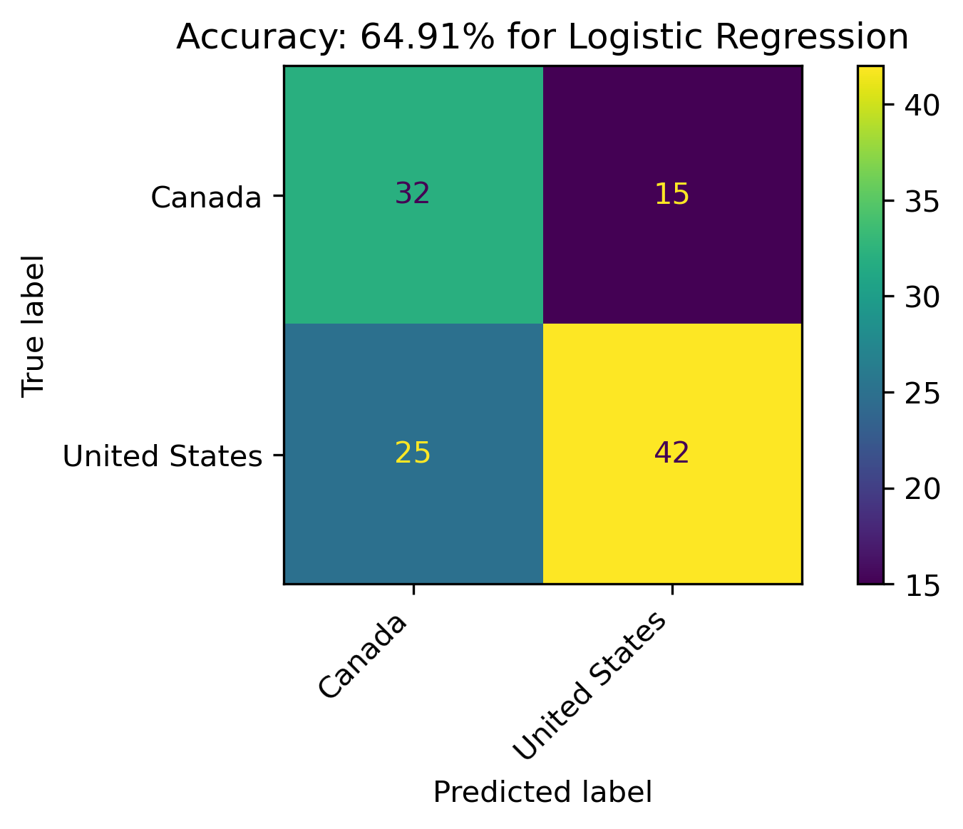
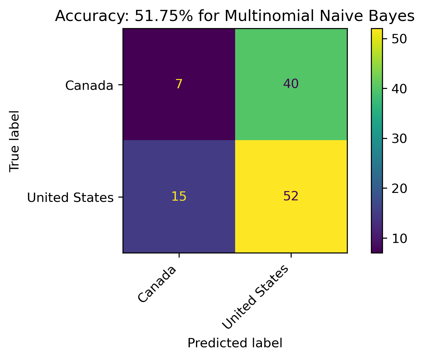
The models resulted in the following accuracies:
- Logistic Regression: 64.91%
- Multinomial Naive Bayes: 51.75%
As explained in the introduction to this section, Logistic Regression is actually a classification technique. For this data, it performs better than Multinomial Naive Bayes.
Conclusion
The aim of this analysis was to investigate if selected characteristics of ski resorts provided information into which country the ski resort was located in. Number of lifts and number of trails by difficulty for ski resorts were examined in comparison to their respective countries. A moderate significance was found, however there was indication that the selected characteristics tended to suggest different countries. Perhaps different characteristics or further categories, such as an investigation into the finer scale of regions would find greater significances.